attention-variants
February 06, 2025
This article explains three popular attention variants:
- Flash Attention
- Paged Attention (used by vLLM)
- Multi-head Latent Attention (used by deepseek)
Flash Attention
The aim of flash attention is to compute attention result with fewer IO and memory storage, and faster computation.
Reference: https://arxiv.org/pdf/2205.14135
The main idea is to split the inputs $Q, K, V$ into blocks, load them from slow HBM to fast SRAM, then compute the attention output with respect to those blocks.
For GPU, there are
- High Bandwidth Memory (HBM): GPU main memory, e.g., 32 GB for GeForce 5090
- Static Random-Access Memory (SRAM): memory per GPU core, e.g., GeForce 5090, L1 Cache: 128 KB (per SM), L2 Cache: 88 MB
Given $Q,K,V \in \mathbb{R}^{n \times d}$, Memory Requirements:
| Standard Attention | Flash Attention | |
|---|---|---|
| Compute $QK^{\top}$ | $n^2 d$ | $nd$ |
| Store $QK^{\top}$ | $n^2$ | None |
| Apply Softmax | $n^2$ | $n$ |
| Multiply by $V$ | $n^2d$ | $nd$ |
| Attention Output | $n^2$ | $n$ |
Flash Attention In Detail
Given $Q,K,V \in \mathbb{R}^{n \times d}$, a standard attention can be written as
\[\begin{align*} S &= Q K^{\top} \in \mathbb{R}^{n \times n} \\ P &= \text{Softmax}(S) \\ A &= PV \in \mathbb{R}^{n \times d} \end{align*}\]Often, there is $n \gg d$ (e.g., for GPT2, $n=1024$ and $d=64$). Attention score $S=Q K^{\top}$ has a large size if the row $n$ is large.
Matrix multiplication can be sliced and fit into CUDA cores, however, softmax $P=\text{Softmax}(S)$ needs the entire row of scores to compute and this step is not linear hence not able to get sliced.
To solve this, Flash Attention keeps running statistics for:
- $m_i$ The maximum value in each row (to prevent overflow in softmax).
- $z_i$ The sum of exponentials in each row (to normalize the softmax).
In other words, the softmax computation is approximated with the help of $m_i$ and $z_i$ without mandating an entire row be joined at once. The softmax approximation in flash attention iteratively updates
Tiling and Algo Process
Flash Attention avoids storing the entire $S$ matrix by computing it tile by tile (or block by block). This is known as tiling.
Flash attention splits $n$ rows into multiple blocks $Q_i \in \mathbb{R}^{b_r \times d}$ and $K_j, V_j \in \mathbb{R}^{b_c \times d}$. $T_r=n/b_r$ and $T_c=n/b_c$ are the numbers of blocks with respects to row and col.
A forward of the flash attention shows as follows (here the index $i$ and $j$ represents block index rather than each row/col)
\[\begin{align*} &\bold{for}\space 1 \le j \le T_c \space\bold{do} \\ &\qquad \text{Load } K_j, V_j \text{ from HBM to on-chip SRAM} \\ &\qquad \bold{for}\space 1 \le i \le T_r \space\bold{do} \\ &\qquad\qquad \text{Load } Q_i, A_i, \bold{m}_i, \bold{z}_i \text{ from HBM to on-chip SRAM} \\ &\qquad\qquad \text{On chip, compute } S_{ij}=Q_iK^{\top}_j \in \mathbb{R}^{b_r \times b_c} \\ &\qquad\qquad \text{On chip, compute } \tilde{\bold{m}}_{ij}=\text{rowmax}(S_{ij})\in\mathbb{R}^{b_r}, \tilde{P}_{ij}=\exp(S_{ij}-\tilde{\bold{m}}_{ij}) \in \mathbb{R}^{b_r \times b_c}, \tilde{\bold{z}}_{ij}=\text{rowsum}(\tilde{P}_{ij}) \in\mathbb{R}^{b_r} \\ &\qquad\qquad \text{On chip, update } \bold{m}_i^{(\text{new})}=\max(\bold{m}_i, \tilde{\bold{m}}_{ij})\in\mathbb{R}^{b_r}, \bold{z}_i^{(\text{new})}=e^{\bold{m}_i-\bold{m}_i^{(\text{new})}}\bold{z}_i+e^{\tilde{\bold{m}}_i-\bold{m}_i^{(\text{new})}}\tilde{\bold{z}}_i\in\mathbb{R}^{b_r} \\ &\qquad\qquad \text{Write back to HBM: } A_i \leftarrow \text{diag}(\bold{z}_i^{(\text{new})})^{-1}\big(\text{diag}(\bold{z}_i)e^{\bold{m}_i-\bold{m}_i^{(\text{new})}}A_i+e^{\tilde{\bold{m}}_i-\bold{m}_i^{(\text{new})}}\tilde{P}_{ij}V_{j}\big) \\ &\qquad\qquad \text{Write back to HBM: } \bold{z}_i \leftarrow \bold{z}_i^{(\text{new})}, \bold{m}_i \leftarrow \bold{m}_i^{(\text{new})} \\ &\qquad \bold{end} \space \bold{for} \\ & \bold{end} \space \bold{for} \\ \end{align*}\]Softmax Approximation Explanation
$S_{ij}=Q_iK^{\top}_j \in \mathbb{R}^{b_r \times b_c}$ only accounts for $b_r$ dims, however, to approximate the full $\text{Softmax}(S_i)$, need full row all elements $n=b_c \times T_c$ included.
To aggregate the $S_{ij}$ for $1 \le i \le T_r$ without storing all elements, max element \(\tilde{\bold{m}}_{ij}\) is computed and iteratively updated \(\bold{m}_i^{(\text{new})}=\max(\bold{m}_i, \tilde{\bold{m}}_{ij})\). The max element \(\bold{m}_i\) of \(S_{ij}\) is a normalization method to prevent overflow such as \(\exp(S_{ij}-\tilde{\bold{m}}_{ij})\le\bold{1}\), and the ensued \(\exp(\bold{m}_i-\bold{m}_i^{(\text{new})})\le\bold{1}\).
\(\text{diag}(\bold{z}_i^{(\text{new})})^{-1}\) is the normalization approximated as denominator of \(\text{softmax}\). $A_i$ is added with the iterative increment \(\tilde{P}_{ij}V_{j}\).
At this iterative step \(i=t\) to write back to HBM to derive \(A_i\), the normalization term \(\text{diag}(\bold{z}_i^{(\text{new})})^{-1}\) accounts for the accumulated \(t\) steps of attention output \(A_{1:t}=\sum_{i=1}^{t}e^{\tilde{\bold{m}}_i-\bold{m}_i^{(\text{new})}}\tilde{P}_{ij}V_{j}\); \(\text{diag}(\bold{z}_i)e^{\bold{m}_i-\bold{m}_i^{(\text{new})}}\) accounts for previous \(t-1\) steps \(A_{1:t-1}\), and \(e^{\tilde{\bold{m}}_i-\bold{m}_i^{(\text{new})}}\) is the scale for this \(t\)-th step \(A_t\).
Memory Efficiency Discussions
Standard Attention Mem Usage
For the computation is sequential, to derive $A$, storage of $S$ and $P$ is necessary.
\[S = Q K^{\top} \in \mathbb{R}^{n \times n} \qquad P = \text{Softmax}(S) \qquad A = PV \in \mathbb{R}^{n \times d}\]- Load $Q,K$ from HBM, compute $S = Q K^{\top}$, write $S$ to HBM: consumed memory $2 \times n \times d + n^2$
- Load $S$ from HBM, compute $P = \text{Softmax}(S)$ and write $P$ to HBM: takes up $n^2$ memory, replacing $S$ with $P$
- load $P$ and $V$ from GBM to compute $A = PV$, write back $A$ to HBM: used memory $n\times d$ for $V$, and $n^2$ for $P$ replaced with the output $A$
In conclusion, it is $O(nd+n^2)$ on HBM access.
Flash Attention Mem Usage
Let $n$ be the sequence length, $d$ be the head dimension, and $M$ be size of SRAM with $d\le M \le n\times d$. Standard attention requires $O(n\times d + n^2)$ HBM accesses, while Flash Attention requires $O(n^2d^2M^{-1})$.
To best utilize SRAM, split $K$ and $V$ to the size relative to $M$, for each block (indexed by $j$) of $K$ and $V$ iterate all blocks (indexed by $i$) of $Q$. The intermediate value computation passes $\frac{n \times d}{M}$ times over $Q$.
For softmax normalization takes into consideration the row only, each row’s softmax is independent from each other, hence $1 \le j \le T_c$ are processed in parallel.
Each pass on $Q$ loads $n \times d$ elements of $K$ and $V$.
Together it is $O(n^2d^2M^{-1})$ on HBM access.
Example
Set use_flash_attention=True.
by 2024, only Nvidia CUDA is supported for flash attention.
import torch
from transformers import AutoModelForCausalLM, AutoTokenizer

# Load a model that supports Flash Attention (e.g., GPT-2 or GPT-NeoX)
model_name = "gpt2"  # Replace with a model that supports Flash Attention
tokenizer = AutoTokenizer.from_pretrained(model_name)
model = AutoModelForCausalLM.from_pretrained(model_name, torch_dtype=torch.float16, device_map="auto")

# Enable Flash Attention (if supported by the model and library)
model.config.use_flash_attention = True

# Input text
text = "Flash Attention is an efficient algorithm for transformers."

# Tokenize input
inputs = tokenizer(text, return_tensors="pt").to("cuda")

# Generate output with Flash Attention
with torch.no_grad():
    outputs = model.generate(**inputs, max_length=50)

# Decode and print the output
print(tokenizer.decode(outputs[0], skip_special_tokens=True))
Paged Attention
Paged Attention is used to host LLMs for high throughput by flexible sharing of key value (KV) cache within and across requests to further reduce memory usage.
Paged Attention is the key technology behind the framework vLLM.
Reference: https://arxiv.org/pdf/2309.06180
Key Value Caches
The key $K$ and value $V$ of the $\text{Attention}(Q,K,V)$ are stored for previous tokens for next token prediction.
For example, assumed model has already processed $128$ tokens, base on which to predict the $129$-th token.
For ONE layer of BERT-base, there is
\[K\in\mathbb{R}^{\text{numHeads}\times\text{seqLen}\times\text{headDim}}=\mathbb{R}^{12\times 128\times 64} \\ V\in\mathbb{R}^{\text{numHeads}\times\text{seqLen}\times\text{headDim}}=\mathbb{R}^{12\times 128\times 64}\]These caches are maintained per layer. Thus, there are $12$ independent pairs of caches (one pair per layer).
For 4k context length with FP16, there is KV cache $2 \times 12 \times 12\times 4096\times 64 \times 2\text{bytes}=144\text{MB}$.
KV Cache Memory Usage Issues and Motivations
KV Caches are stored in contiguous memory, however, such caches dynamically grow and shrink over time as the model generates new tokens (next prediction token is dependent on previous ones), and its lifetime and length are not known a priori.
There are two problems to address:
- Lots of memory fragmentation
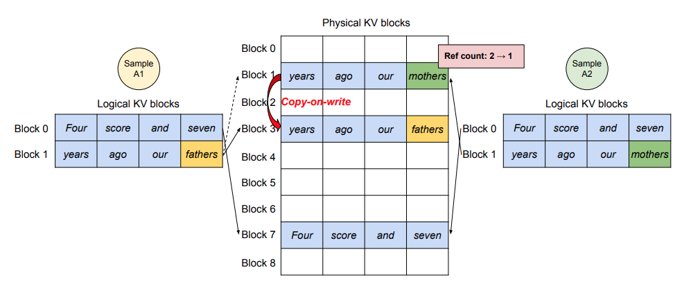
- Memory sharing, e.g., parallel sampling and beam search
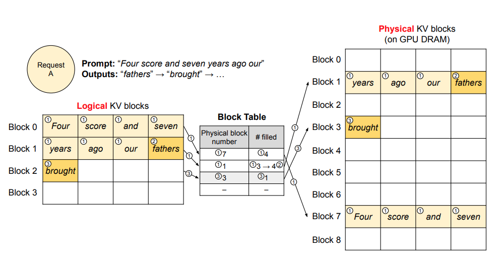
Paged attention maintains a lookup table that KV caches are stored in individual non-contiguous blocks.
</br>
Improvement Examples by Storing KV Caches in Blocks
Top-K Parallel Sampling
No need of memory re-allocation for the KV cache for just one token selection among candidate tokens.
</br>
Prompt Sharing
Many user prompts share a prefix, thus the LLM service provider can store the KV cache of the prefix in advance to reduce the redundant computation spent on the prefix.
Multi-Head Latent Attention (MLA)
Multi-Head Latent Attention (MLA) proposes low-rank key-value joint compression to reduce KV Cache memory. DeepSeekV2 and DeepSeekV3 uses MLA.
Reference: https://arxiv.org/pdf/2405.04434
Notice $K$ and $V$ memory consumption grows as context length grows. The MLA attempts to compress the cached $K$ and $V$ with a low-rank joint compression matrix $C$.
Derive the compression matrix $C$
Let $\bold{h}_t\in\mathbb{R}^{d}$ be the input to an attention layer, where $d=n_h\times d_h$ is the embedding dimension in which $n_h$ is the number of attention heads, and $d_h$ is the dimension per head.
Preliminaries: Standard Multi-Head Attention
For standard multi-head attention, $\bold{q}_t, \bold{k}, \bold{v}_t$ are computed by linear projection from $\bold{h}_t$, and sliced into $n_h$ heads/blocks.
\[\begin{align*} [\bold{q}_{t,1};\bold{q}_{t,2};...;\bold{q}_{t,n_h}]=\bold{q}_t=W^{Q}\bold{h}_t \\ [\bold{k}_{t,1};\bold{k}_{t,2};...;\bold{k}_{t,n_h}]=\bold{k}_t=W^{K}\bold{h}_t \\ [\bold{v}_{t,1};\bold{v}_{t,2};...;\bold{v}_{t,n_h}]=\bold{v}_t=W^{V}\bold{h}_t \\ \end{align*}\]The sliced $\bold{q}_t, \bold{k}, \bold{v}_t$ are used for the multi-head attention computation.
\[\begin{align*} \bold{o}_{t,i} &= \sum_{j=1}^{t} \text{softmax}_j\Big(\frac{\bold{q}^{\top}_{t,i}\bold{k}_{j,i}}{\sqrt{d_h}}\Big)\bold{v}_{j,i} \\ \bold{o}_{t} &= W^{O}[\bold{o}_{t,1};\bold{o}_{t,2};...;\bold{o}_{t,n_h}] \end{align*}\]where $[…]$ is a concatenation operator.
Add Compression Cache Matrices
Add a down-projection matrix $W^{\text{Down-}KV}$ to generate the KV cache $\bold{c}_t^{KV}$, by which add two up-projection matrices to restore $K$ by $W^{\text{up-}K}$ and $V$ by $W^{\text{up-}V}$ to full multi-head dimension: $\bold{k}_t^{C},\bold{v}_t^{C}\in\mathbb{R}^{n_h d_h}$.
During inference, MLA only needs to cache $\bold{c}_t^{KV}$.
\[\begin{align*} \bold{c}_t^{KV} &= W^{\text{Down-}KV}\bold{h}_t \\ \bold{k}_t^{C} &= W^{\text{Up-}K}\bold{c}_t^{KV} \\ \bold{v}_t^{C} &= W^{\text{Up-}V}\bold{c}_t^{KV} \\ \end{align*}\]where $\bold{c}_t^{KV}\in\mathbb{R}^{d_c}$ is the compressed latent vector for keys and values such that $d_c\ll d_h n_h$. This shows that the token cache $\bold{c}_t^{KV}$ compresses the token’s multi-head vectors into a small encoding.
$W^{\text{Up-}K}, W^{\text{Up-}V} \in\mathbb{R}^{d_h n_h \times d_c}$ restore the key $K$ and value $V$ to full dimension $d=d_h \times n_h$.
Also perform low-rank compression for the queries (this is for training):
\[\begin{align*} \bold{c}_t^{Q} &= W^{\text{Down-}Q}\bold{h}_t \\ \bold{q}_t^{C} &= W^{\text{Up-}Q}\bold{c}_t^{Q} \\ \end{align*}\]Decoupled Rotary Position Embedding (RoPE) for KV Restoration
Empirical study by DeepSeek found high importance of positional info, considered $\text{RoPE}$ be introduced.
RoPE is position-sensitive for both keys and queries, that only $Q$ and $K$ are applied RoPE.
\[\begin{align*} [\bold{q}_{t,1}^{\text{Ro}};\bold{q}_{t,2}^{\text{Ro}};...;\bold{q}_{t,n_h}^{\text{Ro}}]=\bold{q}_{t}^{\text{Ro}}=\text{RoPE}(W^{\text{Ro-}Q}\bold{c}_t^Q) \\ \bold{k}_{t}^{\text{Ro}}=\text{RoPE}(W^{\text{Ro-}K}\bold{h}_t) \\ \end{align*}\]Accordingly, the $Q$ and $K$ are
\[\begin{align*} \bold{q}_{t,i}=[\bold{q}_{t,i}^{\text{C}};\bold{q}_{t,i}^{\text{Ro}}] \\ \bold{k}_{t,i}=[\bold{k}_{t,i}^{\text{C}};\bold{k}_{t}^{\text{Ro}}] \\ \end{align*}\]Notice here \(\bold{k}_{t,i}=[\bold{k}_{t,i}^{\text{C}};\bold{k}_{t}^{\text{Ro}}]\) for each token key head \(\bold{k}_{t,i}\) share the same key \(\bold{k}_{t}^{\text{Ro}}\).
Motivation: The non-commutative RoPE
Recall the $QK^{\top}$ definition that for the attention score of the token $t$, it can be decomposed into $\Big(W^{Q}\bold{h}_t\Big)\Big(W^{K}\bold{h}_t\Big)^{\top}$.
Then introduce compression, there is $\Big(W^{Q}\bold{h}_t\Big)\Big(W^{\text{Up-}KV}W^{\text{Down-}KV}\bold{h}_t\Big)^{\top}$. Recall that $\bold{c}_t^{KV}=W^{\text{Down-}KV}\bold{h}_t\in\mathbb{R}^{d_c}$ is quite small in dimension length compared to the full dimension multiplication $W^{\text{Up-}KV}W^{\text{Down-}KV}\bold{h}_t\in\mathbb{R}^{d}$, it can be arranged that $W^{Q}{(W^{\text{Up-}KV})}^{\top}\bold{h}_t$ be absorbed together in matrix multiplication to reduce memory footprint.
\[\underbrace{\Big(W^{Q}\bold{h}_t\Big)}_{\bold{q}_t\in\mathbb{R}^{d}}\Big(W^{\text{Up-}KV}W^{\text{Down-}KV}\bold{h}_t\Big)^{\top} \quad\Rightarrow\quad \underbrace{\Big(W^{Q}{(W^{\text{Up-}KV})}^{\top}\bold{h}_t\Big)}_{\bold{q}_t\in\mathbb{R}^{d_c}} \Big(W^{\text{Down-}KV}\bold{h}_t\Big)^{\top}\]However, if added RoPE, the above linear matrix multiplication does not hold for matrix multiplication does not follow commutative rules.
Introduce RoPE to keys: $\Big(W^{Q}\bold{h}_t\Big)\Big(\text{RoPE}\big(W^{\text{Up-}KV}W^{\text{Down-}KV}\bold{h}_t\big)\Big)^{\top}$.
But RoPE cannot commute with $W^{\text{Up-}KV}$:
\[\Big(W^{Q}\bold{h}_t\Big)\Big(\text{RoPE}\big(W^{\text{Up-}KV}...\big)\Big)^{\top} \quad\not\Rightarrow\quad \Big(W^{Q}\big(\text{RoPE} \cdot W^{\text{Up-}KV}\big)^{\top}\bold{h}_t\Big)\Big(...\Big)^{\top}\]Solution: Decoupled RoPE to query and key
The solution is to decouple RoPE by adding additional multi-head queries \(\bold{q}_{t,i}^{\text{Ro}}\in\mathbb{R}^{d^{\text{Ro}}_h}\) and a shared key \(\bold{k}_{t}^{\text{Ro}}\in\mathbb{R}^{d^{\text{Ro}}_h}\) to carry RoPE.
Introduce \(W^{\text{Ro-}Q}\in\mathbb{R}^{d^{\text{Ro}}_hn_h\times d_c^Q}\) and \(W^{\text{Ro-}K}\in\mathbb{R}^{d^{\text{Ro}}_h\times d}\).
\[\begin{align*} [\bold{q}_{t,1}^{\text{Ro}};\bold{q}_{t,2}^{\text{Ro}};...;\bold{q}_{t,n_h}^{\text{Ro}}]=\bold{q}_{t}^{\text{Ro}}=\text{RoPE}(W^{\text{Ro-}Q}\bold{c}_t^Q) \\ \bold{k}_{t}^{\text{Ro}}=\text{RoPE}(W^{\text{Ro-}K}\bold{h}_t) \\ \end{align*}\]Accordingly, the $Q$ and $K$ are
\[\begin{align*} \bold{q}_{t,i}=[\bold{q}_{t,i}^{\text{C}};\bold{q}_{t,i}^{\text{Ro}}] \\ \bold{k}_{t,i}=[\bold{k}_{t,i}^{\text{C}};\bold{k}_{t}^{\text{Ro}}] \\ \end{align*}\]Let $l$ be history output token number, MLA requires a total KV cache containing $(d_c+d^{\text{Ro}}_h)l$ elements.
Final: Combine the Cache and RoPE
For each token, the attention is
\[\begin{align*} \bold{q}_{t,i} &=[\bold{q}_{t,i}^{\text{C}};\bold{q}_{t,i}^{\text{Ro}}] \\ \bold{k}_{t,i} &=[\bold{k}_{t,i}^{\text{C}};\bold{k}_{t}^{\text{Ro}}] \\ \bold{o}_{t,i} &= \sum_{j=1}^{t} \text{softmax}_j\Big(\frac{\bold{q}^{\top}_{t,i}\bold{k}_{j,i}}{\sqrt{d_h+d^{\text{Ro}}_h}}\Big)\bold{v}_{j,i}^C \\ \bold{o}_{t} &= W^{O}[\bold{o}_{t,1};\bold{o}_{t,2};...;\bold{o}_{t,n_h}] \end{align*}\]