Bond and Repurchase Agreement (REPO) Quant Basics
April 24, 2025
Bond Issuance
When a company needs financing (500 mil), it issues bond by credit. Then financial institutions bid to help bond issuance with proposed rates.
| Institutions | Proposed Rates | Quantity (million) |
|---|---|---|
| Institution A | 3.975% | 150 |
| Institution B | 4.00% | 100 |
| Institution C | 3.95% | 250 |
Financial institutions will pay cash to the company, then distribute the bond per each 100 face value to individual clients.
Bond Related Trading
- Bond trading
- Repurchase Agreement (REPO) (by pledge)
- Repurchase Agreement (REPO) (outright)
- Bond buy/sell back
Bond Types
Classification by Interest Payment
- Fixed-Rate Bonds
Interest Payment: Pay a fixed interest rate (coupon) periodically (usually semi-annually or annually).
- Floating-Rate Bonds (FRBs)
Interest Payment: Pay variable interest linked to a benchmark rate (e.g., LIBOR, SOFR, EURIBOR) plus a fixed spread.
- Zero coupon bonds
Interest Payment: No periodic interest. Issued at a discount and redeemed at face value.
- Step-up/down bonds
Step-Up Bonds: Interest rate increases at predefined intervals.
Step-Down Bonds: Interest rate decreases over time.
- Deferred interest bonds
Interest Payment: No interest paid for an initial period; then periodic payments begin.
- Payment-in-Kind (PIK) Bonds
Interest Payment: Pay interest in additional bonds or equity instead of cash.
Classification by Credibility
- Rate/Govt Bond
Govt bonds are usually high quality, seldomly default
- Credit/Corp Bond
Corp bonds have higher risks of default
Bond Basic Stats
- Coupon Factor
The Factor to be used when determining the amount of interest paid by the issuer on coupon payment dates.
- Coupon Rate
The interest rate on the security or loan-type agreement, e.g., $5.25\%$. In the formulas this would be expressed as $0.0525$.
- Day Count Factor
Figure representing the amount of the Coupon Rate to apply in calculating Interest.
- Pool factor
A pool factor is the outstanding principle out of the amount of the initial principal for ABS or MBS.
\[F_{pool} = \frac{\text{OutstandingPrincipleBalance}}{\text{OriginalPrincipleBalance}}\]E.g., $F_{pool}=0.4$ for \$1,000,000 loan means the underlying mortgage loan that remains in a mortgage-backed security transaction is \$400,000, and \$600,000 has been repaid.
Day Count Factor: Day count Conventions
A day count convention determines how interest accrues over time.
In U.S., there are
- Actual/Actual (in period): T-bonds
- 30/360: U.S. corporate and municipal bonds
- Actual/360: T-bills and other money market instruments (commonly less than 1-year maturity)
Terminologies in Bonds
Bond Issue Price/Size/Factor
- Issue Price
Usually, issue price for a bond is $100$ same as bond face value. However, some zero-coupon bonds have $\text{IssuePrice}<100$.
It can be used for profit and tax calculation.
\[\begin{align*} \text{profit}&=100-\text{issuePrice} \\ \text{withholdingTax}&=\text{profit} \times \text{taxRate} \end{align*}\]- Issue Size
Total bond issuance size.
An individual trader’s position of a bond indicates how much exposure/manipulation he/she is to the market. For example, if a trader has a high position of a bond $\frac{\text{traderThisBondPosition}}{\text{thisBondTotalIssueSize}}>90\%$, he/she could very much manipulate the price of this bond.
- Issue Factor
A custom discount factor to issue price, usually 100.
Bond Pool Factor
Pool factor is used for amortizing lent securities.
Below code simulates for mortgage-based securities assumed the underlying is fully paid off after 12 months, how pool factor is updated every month.
remaining_principal = original_principal
monthly_rate = annual_interest_rate / 12
monthly_payment = original_principal * (monthly_rate * (1 + monthly_rate)**term_months) / ((1 + monthly_rate)**term_months - 1)
for month in range(0, 12):
    remaining_principal -= monthly_payment
    pool_factor = remaining_principal / original_principal
Bond Value/Price Calculation
- Accrued interest
Accrued interest is the interest on a bond or loan that has accumulated since the principal investment, or since the previous coupon payment if there has been one already.
In other words, the interest accounts for the time since the bond’s start date or the last coupon payment date.
- Clean and dirty price
“Clean price” is the price excluding any interest that has accrued.
“Dirty price” (or “full price” or “all in price” or “Cash price”) includes accrued interest.
\[\text{dirtyPrice}=\text{poolFactor}\times(\text{cleanPrice}+\text{accruedInterest})\]- Value and value factor
A value factor is a custom bond value adjustment factor, usually 100.
\[\text{bondPositionValue}= \text{dirtyPrice} \times \text{Quantity} \div \text{issueFactor} \times \text{valueFactor}\]- Cash Flow and Present Value
Let $C_{t_1},C_{t_2},…,C_{t_n}$ be bond cash flow, the present value estimate is
\[PV=\sum^n_{i=1} C_{t_i} e^{-r(t_i)t_i}\]For example, a three-year maturity bond with 3% annualized coupon rate would see cash flow:
\[C_{t_1}=3,\quad C_{t_2}=3,\quad C_{t_3}=103\]The Three Yield Curves
Definition of The Three Yield Curves
Yield to Maturity (YTM) Curve (到期收益率曲线)
Yield to maturity (YTM) is the rate when bond is purchased on the secondary market, expected annualized return rate.
\[\text{BondPrice}=\sum^n_{t=1}\frac{\text{CouponRate}}{(1+r)^t}+\frac{\text{FaceValue}}{(1+r)^n}\]For example, a two-year maturity, 6% coupon rate bond with a face value of 100 priced at 98 on the market, there is
\[98=\frac{6}{1+r}+\frac{106}{(1+r)^2}, \qquad r\approx 7\%\]YTM Initial State Equivalent
At the time it is purchased, a bond’s yield to maturity (YTM) and its coupon rate are the same.
Spot Rate Curve (即期收益率曲线)
Computed rate for zero coupon bond.
\[PV=\frac{\text{FaceValue}}{(1+r_t)^t}\]For example, given that a zero-coupon bond is traded at 92.46, the equivalent yield rate can be computed as $92.46 \times (1+r)^2=100 \Rightarrow r\approx 4\%$.
For coupon payment bonds, it can be used to evaluate individual discounted cash flow to attest how time could affect the bond value.
For example, on market found same type bond spot rates of three different durations: 1y, 2y and 3y for $r_1=2\%,r_2=3\%,r_3=4\%$, discount each cash flow
\[PV=\frac{5}{1.02^1}+\frac{5}{1.03^2}+\frac{105}{1.04^3}\approx 102.96\]Forward Rate Curve (远期收益率曲线)
Computed rate $f(t_1, t_2)$ for between future timestamps $t_1$ and $t_2$.
\[\big(1+f(t_1, t_2)\big)^{t_2-t_1}= \frac{\big(1+r(t_2)\big)^{t_2}}{\big(1+r(t_1)\big)^{t_1}}\]For example, again a two-year maturity bond of 100 face value is priced at 92.46 when issued. Given that $92.46 \times (1+r)^2=100 \Rightarrow r\approx 4\%$, and trader found that the one year spot rate of this bond on the market is 3%, the forward rate is
\[(1+0.04)^2 = (1+0.03)\times(1+r), \qquad r\approx 5\%\]Continuous Forward Rate Between Any Range
Given forward rate $\big(1+f(t_1, t_2)\big)^{t_2-t_1}=\frac{\big(1+r(t_2)\big)^{t_2}}{\big(1+r(t_1)\big)^{t_1}}$, in continuous compound rate scenario, there is $e^{(t_2-t_1)f(t_1,t_2)}=\frac{e^{t_2 r(t_2)}}{e^{t_1 r(t_1)}}$, hence there is a simple linear formula:
\[\begin{align*} && e^{(t_2-t_1)f(t_1,t_2)} &=\frac{e^{t_2 r(t_2)}}{e^{t_1 r(t_1)}} \\ \Rightarrow && e^{(t_2-t_1)f(t_1,t_2)}&=e^{t_2 r(t_2)-t_1 r(t_1)} \\ \text{take log } \Rightarrow && (t_2-t_1)f(t_1,t_2) &=t_2 r(t_2)-t_1 r(t_1) \\ \Rightarrow && f(t_1,t_2) &=\frac{t_2 r(t_2)-t_1 r(t_1)}{t_2-t_1} \end{align*}\]P.S., continuous form from discrete is given from an interest rate $r$ assumed the payment number $n$, that $r/n$ means the interest is paid in $n$ times each time payment is $r/n$, there is $\lim_{n\rightarrow\infty}(1+\frac{r}{n})^{nt}=e^{rt}$
Relationship of Spot Rate vs Forward Rate
Instantaneous forward rate $f(t)$ can be defined as forward rate at the moment $t$.
\[f(t)=\lim_{\Delta t \rightarrow 0} \frac{f(t, t+\Delta t)}{\Delta t}\]Consider $t_2 r(t_2)-t_1 r(t_1)=\int^{t_2}_{t_1} f(t)dt$, then at the $t$ moment, the forward rate can be expressed as $r(t)t=\int^t_0 f(u)du$ which is the .
Continuous spot rate growth is
\[\begin{align*} && e^{-r(t)t}&=\exp\Big(-\int^t_0 f(u)du \Big) \\ \text{and instantaneous spot rate is } && r(t) &=\frac{1}{t}\int^t_0 f(u)du \end{align*}\]Spot Rate vs YTM Rate in Bond Valuation
Since spot rate only accounts for zero-coupon bonds, it can be a good interpretation of “time” effect on bond valuation.
YTM is just a weighted average of the various spot rates applied to each cash flow.
Real Example China Bond Spot Rate vs YTM Rate
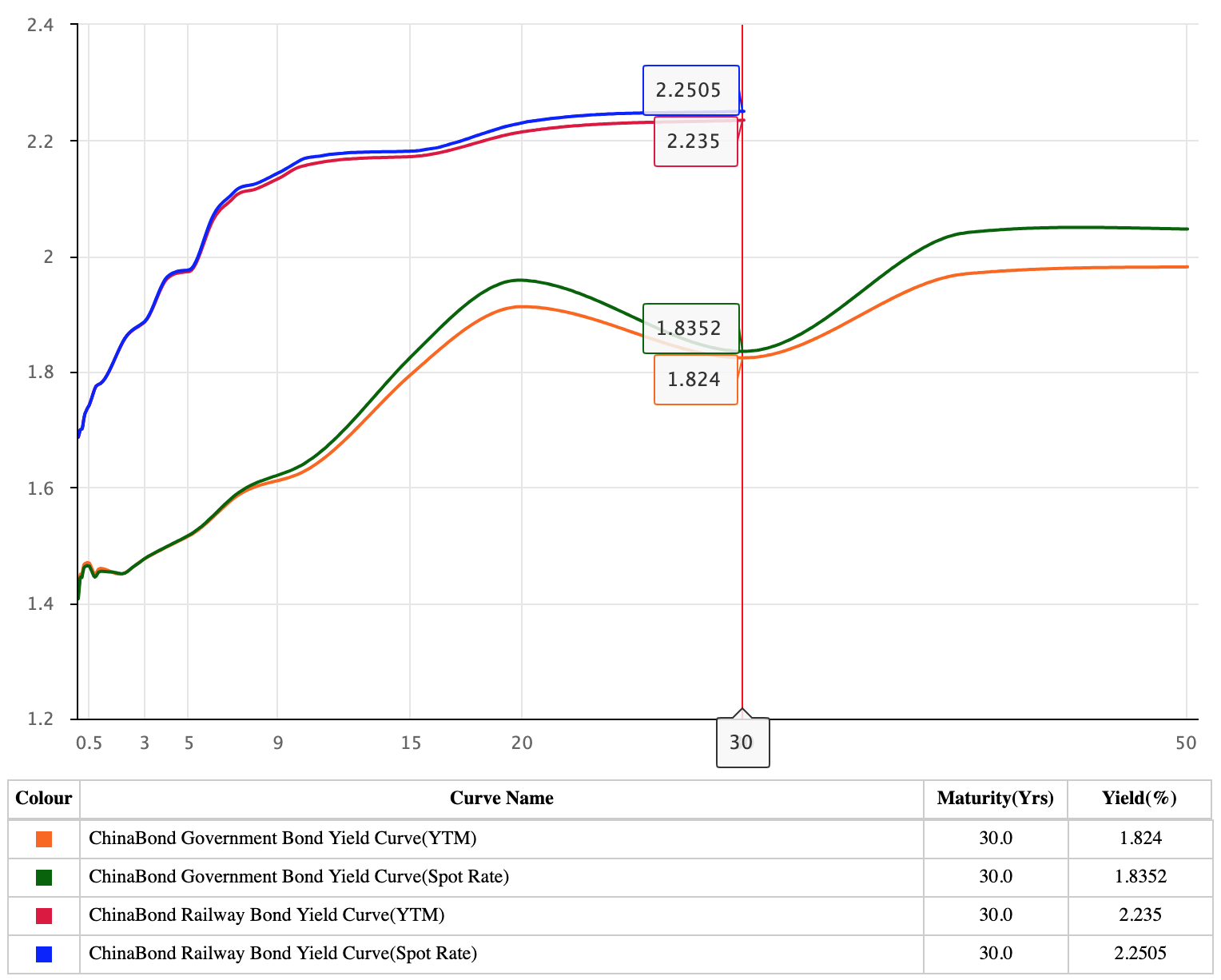
On 2025 May 5, China bond market observes below rate curves.
</br>
In the plot there are two types of bonds: a China corp bond and govt bond, and the corp bond sees higher yield rate than the govt’s.
In early maturity days, YTM and spot rate almost overlap, as market considers likely there is no recent black swan event and the bond will generate cash flow.
Also noticed that at the 30-year maturity point, the YTM and spot rate curves converge. This is a result of 30 year usually picked up as a control point where market agrees as a unified yield.
Why YTM is below spot rate
In summary, upward-sloping spot curves make coupon bond yields (YTM) lower than the final spot rate. Usually investors consider earlier cash flows are relatively more valuable now (long-term duration yields are distrust as investors expect inflation rise).
The heavy weighting of early coupons at lower spot rates depresses the overall YTM below the 30-year spot.
Calculation Example of Spot Rate vs YTM Rate, and Arbitrage-Free Price
Find YTM rate and spot rate of a 3-year 5% coupon face value $1000 bond now traded at $978.12. On market observe that, benchmark (same risk and liquidity, e.g., same company issued bonds) one year annual pay bond at 5.0%, two year benchmark at 5.1% and three year benchmark at 5.5%.
For this bond YTM rate
\[978.12=\frac{50}{1+r}+\frac{50}{(1+r)^2}+\frac{1050}{(1+r)^3},\qquad \Rightarrow r\approx 5.816\%\]Regarding the market benchmark (under the same default and liquidity risk, the overall similar bond yield), it can say that
- benchmark one year annual pay bond’s YTM rate is 5%
- benchmark two year annual pay bond’s YTM rate is 5.1%
- benchmark three year annual pay bond’s YTM rate is 5.5%
For spot rate
Derive each year rate by bootstrapping:
- For the 1st year: $r_1=5\%$
- For the 2nd year: $\frac{5.1}{1.051}+\frac{105.1}{1.051^2}=\frac{5.1}{1.05}+\frac{105.1}{(1+r_2)^2}$, derive $r_2\approx 5.102\%$
- For the 3rd year: $\frac{5.5}{1.055}+\frac{5.5}{1.055^2}+\frac{105.5}{1.055^3}=\frac{5.5}{1.05}+\frac{5.5}{1.05102^2}+\frac{105.5}{(1+r_3)^3}$, derive $r_3\approx 5.524\%$
For arbitrage-free price
\[PV=\frac{5}{1.05}+\frac{5}{1.05102^2}+\frac{105}{1.05524^3}=986.46\]For the bond is priced at $978.12<986.46$, it can be said that the bond is underpriced.
Analysis on Spot Rate vs YTM Rate
YTM rate shows that coupon reinvestment at 5.816% yield (reinvestment yield is identical to YTM) is higher than spot rate between 5.0% - 5.524%. This might be an indicator of default or liquidity risk.
Spot rate shows pure market’s concern of the “time” effect on the bond. The difference between benchmark YTM rate at 5.5% vs bond spot rate 5.524% is traced from market benchmark cash flow by market YTM vs by individual bond spot rates.
Put another way, YTM is just a weighted average of the various spot rates applied to each cash flow
Long-Term Rate Formulation
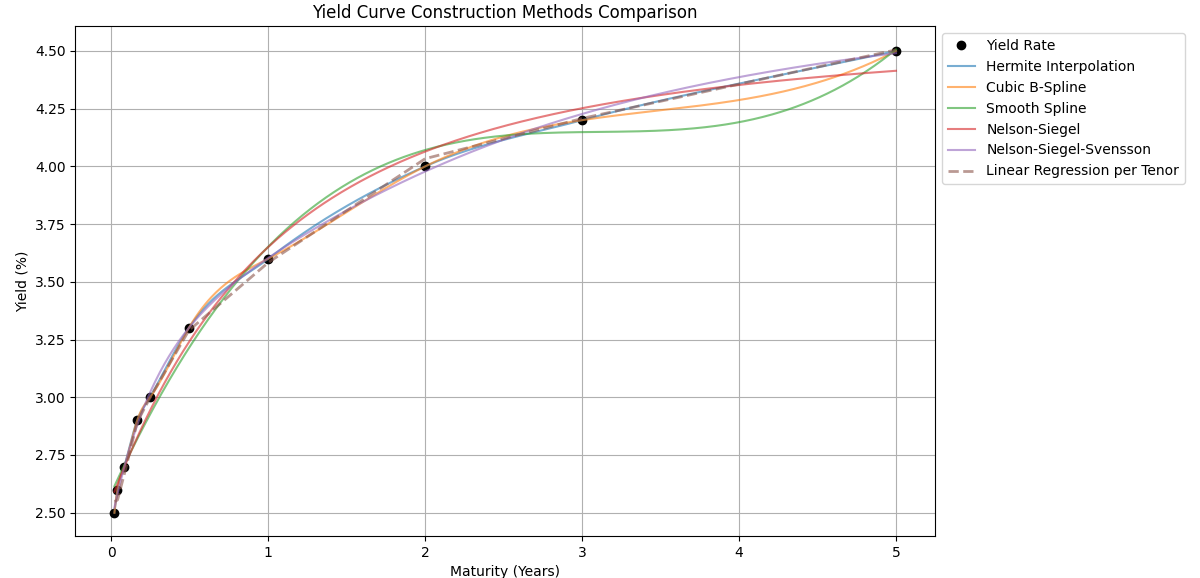
Commonly, there are three categories of curve fitting methods given some spot rates (at fixed durations, e.g., 1y, 3y 5y, 10y) to interpolate rates in between to form a continuous yield curve.
| Method | Characteristics | Use Scenarios |
|---|---|---|
| Bootstrap | Recursively output next predicate based on previous one | Data has fixed discrete tenors to interpolate missing tenors |
| Parametric, e.g., Nelson-Siegel | Parameters have strong economic semantics | Typical use for data with semi-monotonic trends, and data points have different density levels in different ranges |
| Spline | Simply do curve fitting, flexible, but lack economic explanation | If data scatter patterns are likely contained sharp turning corners, while curve smoothness needs to preserve |
Given a set of spot rates, the interpolated curves are shown as below.
</br>
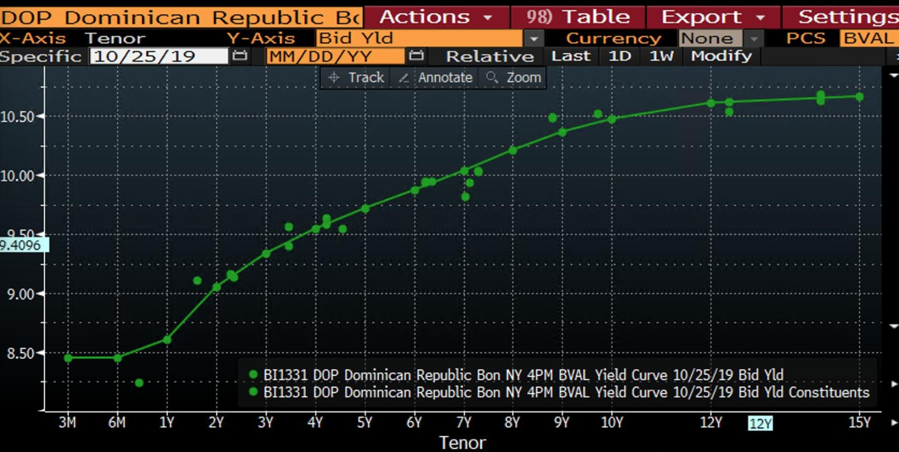
Long-Term Rate Interpolation Example Use Cases
Dominican Republic govt bonds have low liquidity hence parametric method is used for curve interpolation. The large deviation is a sign of low liquidity.
</br>
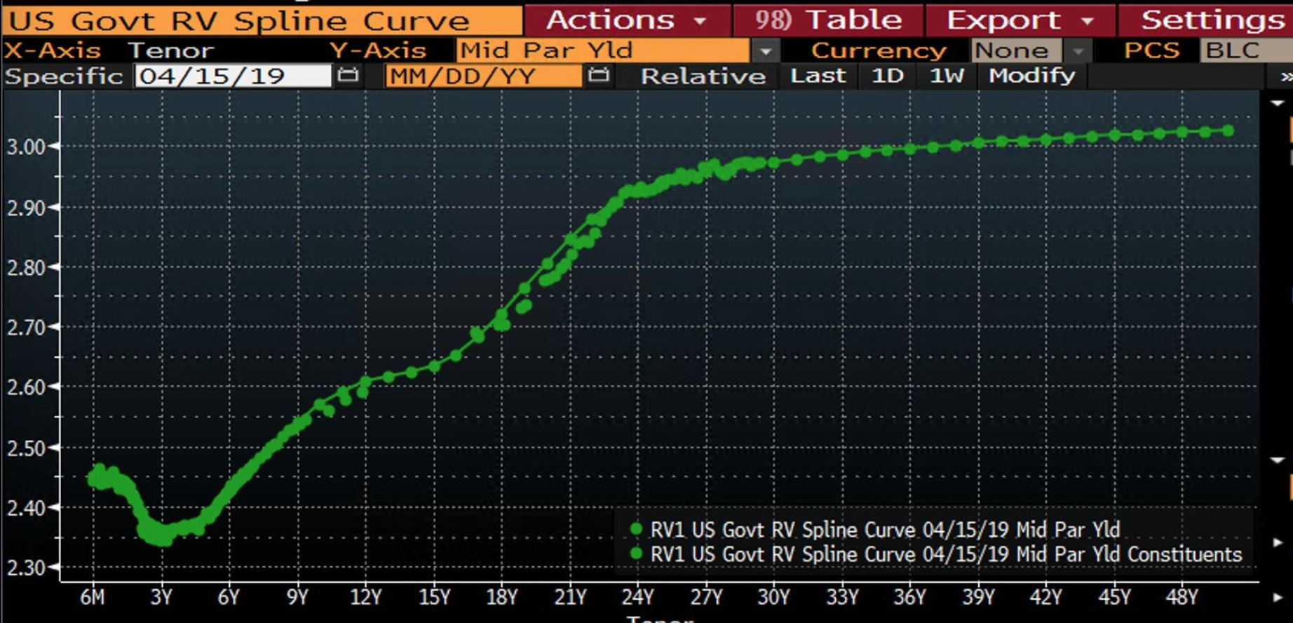
Spline can give a curve shape even if it is NOT monotonic.
</br>
Interpolation In Detail
The below explanations are under the notations/assumptions:
- Let $t$ be the to-be interpolated x-axis points and $t_i$ be the existing points that map the y-axis control points $P_i=f(t_i)$.
Bootstrap
Given dirty prices of different maturity bond from the same issuer, to plot the yield curve, one can use bootstrap to recursively output next maturity spot rate.
Let $C$ be coupon payment and $F$ be face value.
- Compute $r_1$ for 1 year maturity spot rate
- Having obtained $r_1$, then compute $r_2$ for 2 year maturity spot rate
- Having obtained $r_2$, then compute $r_3$ for 3 year maturity spot rate
Hermite Interpolation
$H(t)$ is a polynomial that satisfies $H(t_i)=f(t_i)$ and $\frac{d}{d t_i}H(t_i)=\frac{d}{d t_i}f(t_i)$. Let $t=\frac{t-t_i}{t_{i+1}-t_i}$ be a normalized local variable ($0<t<1$) between $(t_i, t_{i+1})$.
\[H(t)=h_{00}(t)\cdot f(t_{i}) + h_{01}(t)\cdot f(t_{i+1}) + h_{10}(t)\cdot \frac{d}{d t_i}f(t_{i}) + h_{11}(t)\cdot \frac{d}{d t_{i+1}}f(t_{i+1})\]where
\[\begin{align*} h_{00}(t)&=2t^3-3t^2+1 \\ h_{01}(t)&=-2t^3+3t^2 \\ h_{10}(t)&=t^3-2t^2+t \\ h_{11}(t)&=t^3-t^2 \\ \end{align*}\]$H(t_{i+1})=f(t_i)$ mandates that the fitting curve must pass through the control points $P_i=f(t_i)$.
The gradient computation $\frac{d}{d t_i}H(t_i)=\frac{d}{d t_i}f(t_i)$ is at the discretion of user.
A common two-step differential method is (used by numpy.gradient)
where $h$ is the step span.
Fisher-Nychka-Zervos Cubic B-Spline (3B)
Given four control points $P_i,P_{i+1},P_{i+2},P_{i+3}$
\[S(t)=\sum^n_{i=0} P_i \cdot N_{i,3}(t)\]where
\[N_{i,k}(t) = \frac{x - t_i}{t_{i+k} - t_i} N_{i,k-1}(t) + \frac{t_{i+k+1} - x}{t_{i+k+1} - t_{i+1}} N_{i+1,k-1}(t), \qquad k=3\]In detail for $k=3$,
\[\begin{align*} N_{i-3,3}(t)&=\frac{1}{6}(1-t)^3 \\ N_{i-2,3}(t)&=\frac{1}{6}(3t^3+6t^2+1) \\ N_{i-1,3}(t)&=\frac{1}{6}(-3t^3+3t^2+3t+1) \\ N_{i,3}(t)&=\frac{1}{6}t^3 \\ \end{align*}\]Smooth Spline
Define natural cubic spline:
\[f_i(t)=a_i+b_i(t-t_i)+c_i(t-t_i)^2+d_i(t-t_i)^3\] \[\text{subject to }\qquad \frac{d^2}{dt^2}f_i(t_0)=\frac{d^2}{dt^2}f_i(t_n)=0\]that the constraint makes sure the second derivative is zero for the first and end control points.
Add $\lambda$ as smooth control hyper-parameter.
Optimize $f$ by
\[\min_{f}\quad \underbrace{\sum^n_{i=1}\big(P_i-f(t_i)\big)^2}_{\text{deviation penalty}} + \lambda \underbrace{\int\Big(\frac{d^2}{dx^2}f_i(t_n)\Big)^2 dx}_{\text{sharp penalty}}\]where the $\text{deviation penalty}$ encourages the trained $f(t)$ to be as much close as possible to the control point $P_i$ when passing through $f(t_i)$. The $\text{sharp penalty}$ encourages smooth transition as the function $f(t)$ curves (penalize large 2nd order derivatives).
Nelson-Siegel (NS) and Nelson-Siegel-Svensson (NSS)
Assume instantaneous forward rate at a future moment is
\[f(t)=\beta_0+\beta_1 e^{-t/\tau_1}+ \beta_2\frac{t}{\tau_1} e^{-t/\tau_1}\]where
- $\beta_0$ represents long-term convergence rate, encapsulated the overall market expectation for economy.
- $\beta_1$ represents short-term fluctuation how much it deviates from $\beta_0$; when $\tau_1\rightarrow 0$, forward rate collapses to $\beta_0+\beta_1$
- $\beta_2$ is used to control curvature that reaches its max when $t=\tau_1$
- $\tau_1$ is a mid-term factor, larger the value, the longer the mid-term impact lasting; some academics write $\lambda_1=1/\tau_1$ as a wavelength form
Integrate instantaneous rate $f(t)$, the result is
\[\begin{align*} && r(t)&=\beta_0+(\beta_1+\beta_2)\frac{\tau_1}{t} (1-e^{-t/\tau_1})- \beta_2 e^{-t/\tau_1} \\ \text{or}\quad && &=\beta_0+\beta_1\Big(\frac{1-e^{\lambda_1 t}}{\lambda_1 t}\Big)+\beta_2\Big(\frac{1-e^{\lambda_1 t}}{\lambda_1 t}-e^{-\lambda_1 t}\Big) \end{align*}\]Svensson in 1994 added a new set of parameters:
\[r(t)=\beta_0+\beta_1\Big(\frac{1-e^{\lambda_1 t}}{\lambda_1 t}\Big)+\beta_2\Big(\frac{1-e^{\lambda_1 t}}{\lambda_1 t}-e^{-\lambda_1 t}\Big)+\beta_3\Big(\frac{1-e^{\lambda_2 t}}{\lambda_2 t}-e^{-\lambda_2 t}\Big)\]| NS | NSS | |
|---|---|---|
| Parameters | $\beta_0,\beta_1,\beta_2,\lambda_1$ | $\beta_0,\beta_1,\beta_2,\beta_3,\lambda_1,\lambda_2$ |
| Curve shape | Max single peak | Max multiple Peaks |
Short Rate (短期利率) Formulation
Short rate is used to estimate short-term price fluctuation.
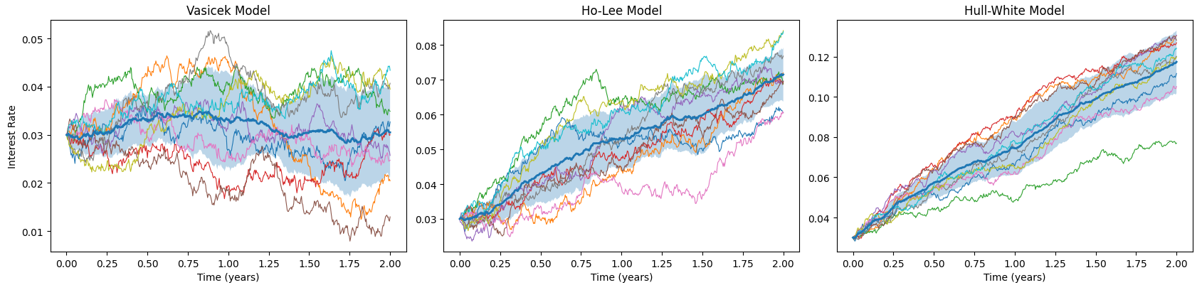
</br>
Visicek Model
The dynamics of short rate can be formulated as an Ornstein-Uhlenbeck (OU) process.
\[d r_t=\theta(\mu-r_t)dt+\sigma dW_t\]where
- $W_t$ is Brownian motion
- $\sigma$ is a diffusion term
- $\mu$ is a drift term
- $\theta$ is the convergence speed $r_t$ approaches to $\mu$ as time goes by
The analytic solution is (integrate over time range $[0,t]$)
\[r_t=\mu \big(1-e^{-\theta t}\big)+r_{0}e^{-\theta t}+ \sigma\int^{t}_{0}\big(e^{-\theta (t-u)}\big)dW_u\]Ho-Lee Model
Ho-Lee model considers using $\theta_t=\frac{\partial f(0,t)}{\partial t}+\sigma^2 t$ as time-dependent drift.
\[d r_t=\theta_t dt+\sigma dW_t\]where
- $W_t$ is Brownian motion
- $\sigma$ is a diffusion term
- $\theta_t=\frac{\partial f(0,t)}{\partial t}+\sigma^2 t$ is a function of $t$ to align with spot rate on the market, where $f(0,t)$ is the forward rate at the initial state
Deduction of $\theta_t$ by No Arbitrage Condition
This expression $\theta_t=\frac{\partial f(0,t)}{\partial t}+\sigma^2 t$ states that the drift term is determined by forward rate and fluctuation $\sigma^2 T$. $f(0,t)$ is the forward rate at the initial state.
\[\begin{align*} \int_0^T r_u du &= \int_0^T r_0 du + \int_0^T\int_0^t \theta_u du dt + \sigma\int_0^T\int_0^t dW_u dt \\ &= r_0 T + \int_0^T\int_0^t \theta_u du dt + \underbrace{\sigma\int_0^T (T-u) dt}_{\sim N(0, \sigma^2\int_0^T(T-u)^2 du)} \end{align*}\]where $\sigma^2\int_0^T(T-u)^2 du=\frac{\sigma^2}{3}T^3$.
The valuation of a bond till $T$ maturity can be written as $P(0,T)=E\left[e^{-\int_0^T r_t dt}\right]$, $\theta_t$ can be deduced as such
\[\begin{align*} && P(0,T)&=E\left[e^{-\int_0^T r_t dt}\right] \\ && &=\exp\bigg(E\left[-\int_0^T r_u du\right]+\frac{1}{2}Var\left[-\int_0^T r_u du\right]\bigg) \\ && &= \exp\bigg(-r_0 T - \int_0^T\int_0^t \theta_u du dt + \frac{\sigma^2}{6}T^3\bigg) \\ \Rightarrow && \int_0^T\int_0^t \theta_u du dt &= \ln P(0,T)-r_0 T + \frac{\sigma^2}{6}T^3 \\ \Rightarrow && \int_0^T \theta_u du &= \frac{\partial}{\partial T}\bigg(\ln P(0,T)-r_0 T + \frac{\sigma^2}{6}T^3\bigg) \\ && &= \frac{\partial}{\partial T}\bigg(\ln P(0,T)\bigg)-r_0 + \frac{\sigma^2}{2}T^2 \\ && &= f(0,T)-r_0 + \frac{\sigma^2}{2}T^2 \\ \Rightarrow && \theta_T &=\frac{\partial}{\partial T}\bigg(f(0,T)-r_0 + \frac{\sigma^2}{2}T^2\bigg) \\ && &=\frac{\partial f(0,T)}{\partial T}+\sigma^2 T \end{align*}\]Hull-White Model
Different from Ho-Lee model, Hull-White model added regression to mean value.
\[dr_t = (\theta_t - a r_t) dt + \sigma dW_t\]where
- $W_t$ is Brownian motion
- $\sigma$ is a diffusion term
- $\theta$ is a function of $t$ to align with spot rate on the market
- $a$ mean value convergence speed to long-term rate
The analytic solution is (integrate over time range $[0,t]$)
\[r_t=r_0 e^{-at}+ \int^{t}_{0}e^{-a (t-u)}\theta_u du+ \sigma\int^{t}_{0}\big(e^{-a (t-u)}\big)dW_u\]Repurchase Agreement (REPO)
A repurchase agreement, also known as a repo, RP, or sale and repurchase agreement, is a form of short-term borrowing, mainly in government securities or good-credit corporate bonds.
The dealer sells the underlying security to investors and, by agreement between the two parties, buys them back shortly afterwards, usually the following day, at a slightly higher price (overnight interest).
REPO vs Reverse REPO
To the party selling the security with the agreement to buy it back, it is a repurchase agreement (REPO).
To the party buying the security and agreeing to sell it back, it is a reverse repurchase agreement (Reverse REPO).
Repo Types by Management and Ownership
Different underlying management and ownerships have implications of coupon payment to what party, permitted/forbidden re-hypothecation (reuse), what governing legal agreements to use (e.g., what netting methods are allowed), etc.
In this context,
- Buyer: to buy/borrow securities, give out money as interest
- Seller: to sell/lend securities, receive interest as money
REPO Types By Custody Management
| Ownership | Coupon | Legal Agreement | Re-hypothecation | Comments/Key Characteristics | |
|---|---|---|---|---|---|
| Classic/Outright Repo | Full ownership transfer | Retained by Buyer | MRA or GMRA | Allowed (at buyer’s discretion) | Also referred as US-style REPO; most typical REPO; to repurchase at a specified price and on a specified date in the future. |
| Tri-Party/Agency Repo | Managed by tri-party agent | Facilitated by Agent | Tri-Party Agreement | Restricted | Collateral is held in an independent third-party account. |
| Held-In-Custody (HIC) Repo | Temporary to buyer in name only, usually favorable to seller | Retained by Seller | Informal custom agreement | Restricted | The seller receives cash for the sale of the security, but holds the security in a custodial account (might not immediately accessible to the buyer) for the buyer. |
REPO Types By Ownership
| Ownership | Coupon | Legal Agreement | Re-hypothecation | Comments/Key Characteristics | |
|---|---|---|---|---|---|
| Classic/Outright Repo | Full ownership transfer | Retained by Buyer | MRA or GMRA | Allowed (at buyer’s discretion) | Also referred as US-style REPO; most typical REPO; to repurchase at a specified price and on a specified date in the future. |
| Pledge-Style Repo | Collateral by pledge, not full ownership | Retained by Seller | Informal custom agreement | Restricted | Classic REPO but underlying by pledge |
| Sell/Buy-Back | Full ownership transfer | Included when purchased, e.g., by bond dirty price | Informal custom agreement | Allowed (at buyer’s discretion) | Two separate trades: spot sale and forward purchase. |
where in pledge vs outright, although in the scenario of credit default that a seller fails to redeem the lent securities and buyer can exercise the right of disposing/selling the securities, buyer might still need to take legal procedure. This is worrying and time-consuming in contrast to outright REPO.
Reference:
https://www.boc.cn/en/cbservice/cb2/cb24/200807/t20080710_1320894.html#:~:text=It%20means%20a%20financing%20activity,bonds%20to%20the%20repo%20party
Repo Types/Products by Tenor and Business Value
“By business value” aims to give an overview of tailored REPO classification by regulation and custom business needs. In other words, different companies/financial institutions provide different repo products (different tenors/renewal agreements) on markets.
Very often, REPO risks arise from tenor (how long to borrow/lend) and quality of underlying securities (high/low quality bonds). As a result, REPO products are regulated/designed per these two aspects.
Repo Type/Product Examples Stipulated by Authority
Available REPO tenors depend on regulations per country. For example, by 2024, Shenzhen Stock Exchange (SZSE, 深圳证券交易所) states only such tenors are allowed in REPO trading.
| Underlying Bonds | Available Tenors |
|---|---|
| High-quality bonds, e.g., gov bonds | 1,2,3,4,7,14,28,63,91,182,273 days |
| Lower-quality bonds, e.g., corp bonds | 1,2,3,4,7 days |
Repo Type/Product Examples Provided by A Financial Institution
A financial institution can provide tailored REPO agreements to REPO counterparties for trading (of course under authority regulations), giving them flexibility of how to pay coupon, lending/borrowing auto-renewal, purchase with different currencies, etc.
| Governing Document | Underlying Asset | Tenor | Legal Title Transfer | Margining | Business | |
|---|---|---|---|---|---|---|
| Typical Repo/Reverse Repo | GMRA | Gov bonds, Credit, Equity | Open, Overnight ~ 5 years | Yes | Daily | Repo: Deploy bond/equity for cash borrow; Reverse repo: Collateralized cash lending for interest |
| Cross Currency Repo | GMRA | Gov bonds, Credit | Open, Overnight ~ 5 years | Yes | Daily | Mostly USD funding to meet US reserve requirements |
| Extendible/Rollover Repo | GMRA | Gov bonds, Credit, Equity | 3 month start with 1 month increment, 1 year start with 1 month increment, etc | Yes | Daily | Extendible agreement periods, typically every 3 months to renew repo termination date |
| Evergreen Repo | GMRA | Gov bonds, Credit, Equity | Notice period > 30 days | Yes | Daily | Even greater flexible to renew repo termination date |
| Total Return Swap | ISDA/CSA | Gov bonds, Credit, Equity | Open, Overnight ~ 1 years | No | Daily | By Repo + Credit Default Swap (CDS) as the reference asset, borrower can leverage much more money by only paying interest to repo and premium to reference asset third party agency |
| Bond Forward | ISDA/CSA | Gov bonds, Credit | Overnight ~ 8 years | Yes | Daily | Bonds are agreed to be sold at a pre-determined price in the future/mark-to-market value at the forward date. This can mitigate the risk associated with bond price volatility between spot and forward dates. |
| Unsecured Bond Borrowing | GMRA | Gov bonds, Credit, Equity | Overnight ~ 1 years | No | None | Borrower borrows money without providing collateral; they are charged high repo interests |
Global Master Repurchase Agreement (GMRA)
Global Master Repurchase Agreement (GMRA) published by International Capital Market Association (ICMA) is standardized legal agreement used globally for repurchase agreements (repos).
The GMRA covers classic repos, sell/buy-backs, and other similar transactions.
Key Objectives of the GMRA
- Provide a standardized framework for repo transactions.
- Reduce legal and operational risks by clarifying the rights and obligations of both parties.
- Facilitate netting and close-out in the event of default.
Credit Support Annex (CSA)
A Credit Support Annex (CSA) is a document that defines the terms for the provision of collateral by the parties in derivatives transactions, developed by the International Swaps and Derivatives Association (ISDA).
REPO RFQ (报价咨询)
RFQ (Requests For Quotes) is for repo sales/traders asking counterparty sales/traders for his/her quotes for REPO trade and the underlying securities.
For example, a sales asks a counterparty trader/sales:
Show your bid on ISIN US12345678JK USD 5mm for 2mth and 3mth
The counterparty trader/sales replies:
My bid for US12345678JK:
5mm 2mth 5hc 3.5%
5mm 3mth 5hc 3.7%
that the RFQ requester wants to sell (requester offer <—> responser bid) USD 5mm (5 million) worth of US12345678JK by dirty price.
The reply shows the trader/sales is willing to bid with haircut discount by 5% and paid interest rate of 3.5% and 3.7% for borrowing US12345678JK for 2 months and 3 months.
The longer the borrowing period, the higher risk of the repo trade, hence the higher interest rate the lending party might charge.
REPO RFQ Types
Outright REPO 买断式回购
The seller (borrower) transfers ownership of the securities to the buyer (lender) with an agreement to repurchase them at a specified price/rate and on a specified date in the future.
Implications: they can sell or reuse the securities (e.g., for further collateralization or trading).
AON (All-or-None, 全部或零)
AON (All-or-None) is a trading condition where an order must be executed in its entirety or not at all.
If the entire order cannot be filled at the specified price or quantity, the order is canceled.
Repo Market Players
- Investors
Cash-rich institutions; banks and building societies
- Borrowers
Traders; financing bond positions, etc
- Tri-Party
Tri-Party is a third-party agent (the tri-party agent) intermediates between two primary parties: the collateral provider (borrower) and the collateral receiver (lender).
Tri-party agent can help increase operational efficiency and flexibility, improve liquidity, and mitigate default risks, for collateral allocation and management, settlement and custody, valuation and margining services are provided by the tri-party agent.
Popular try-party agents are
-> Euroclear (A leading provider of triparty services in Europe)
-> Clearstream
Business Motivations
Central Bank Control over Money Supply
Central bank is rich in cash and has a large reserve of national bonds, so that it can influence the markets.
- Injecting Liquidity (Reverse Repo):
Central bank buys securities from commercial banks with the promise to sell them back at a predetermined date and price. Commercial banks receive money then by loan to distribute money to the society.
- Absorbing Liquidity (Repo)
Central bank sells securities to the banks with an agreement to buy them back later.
Examples
- The United States Federal Reserve Used Repo for Federal Funds Rate (FFR) Adjustment
Repurchase agreements add reserves to the banking system and then after a specified period of time withdraw them; reverse repos initially drain reserves and later add them back. This tool can also be used to stabilize interest rates (FFR).
- Relationship Between Repo and SOFR
Secured Overnight Financing Rate (SOFR) is a broad measure of the cost of borrowing cash overnight collateralized by Treasury securities with a diverse set of borrowers and lenders;. It is based entirely on transactions (not estimates), hence serving a good alternative to London Inter-Bank Offered Rate (LIBOR).
SOFR reflects transactions in the Treasury repo market, e.g., UST (U.S. Treasury), that in the Treasury repo market, people borrow money using Treasury debt as collateral.
- Central bank uses reverse repo to buy securities from financial institutions (typically state-owned banks) to increase their capital reserve/liquidity
SHANGHAI, Nov 29, 2024 (Reuters) - China’s central bank said on Friday it conducted 800 billion yuan ($110.59 billion) of outright reverse repos in November.
The People’s Bank of China (PBOC) said the repo operations aimed to keep liquidity in the banking system adequate at a reasonable level.
This happened for real estate saw sharp drops in prices that resulted in banks losing money. Feared of banks went bankrupt, PBOC decided to inject temporary liquidity into banks.
Individual Financing Needs
REPO Calculation
- Face Value, and Dirty Price vs Clean Price
The Clean Price is the Mark-To-Market (MTM) price of the bond excluding any accrued interest.
The Dirty Price is the total price that the buyer pays: $\text{DirtyPrice}=\text{CleanPrice}+\text{AccruedInterest}$
\[\text{AccruedInterest}= \frac{\text{CouponPayment}\times\text{DaysSinceLastCouponPayment}}{\text{DaysInCouponPeriod}}\]For example, spotted a bond and a trader wants to buy this bond
- Face Value: $1,000 (i.e., issuer declared price at $1,000 per 1,000 units)
- Annual Coupon Rate: $5\%$
- Coupon Payment Frequency: Semi-annual (i.e., $180$ days per payment)
- Clean Price: $980 (i.e., Mark-To-Market (MTM) bond price excluded accrued interest)
- Days Since Last Coupon Payment: $60$ days
To buy this bond, a trader needs to pay
\[\text{DirtyPrice}= 980+\frac{1}{2}(5\% \times 1,000) \times \frac{60}{180}=988.33\]Face value explained: why clean price is lower than face value ? Clean price should be equal to face value (bond issuer declared price) if market/economy/bond issuer are totally stable, but this scenario is too much of ideal.
For example, below factors affect clean price -> Credit Quality of Issuer: If the creditworthiness of the bond issuer has deteriorated, the perceived risk of the bond increases. -> Time to Maturity: As a bond approaches its maturity date, its price tends to move towards its face value. -> Economy: If high-risk securities such as stocks are experiencing a black swan event, investors would sell-off stocks and bulk-buy bonds as a hedging solution; bond clean price rises as a consequence.
- Initial margin (Haircut)
Initial margin is the excess of cash over securities or securities over cash in a repo or securities at the market price when lending a transaction.
Haircut serves as a discount factor to reflect risk aversion consideration of the bond price fluctuations during the lent period. Hence, the actual lent money is slightly lower than the bond market value.
| Haircut method | Haircut formula |
|---|---|
| Divide | $\text{Haircut}=100\times \frac{\text{CollateralMktValue}}{\text{CashLent}}$ |
| Multiply | $\text{Haircut}=100\times \frac{\text{CashLent}}{\text{CollateralMktValue}}$ |
- Repo vs Sell/Buy Back
| Repo | Sell/Buy Back | |
|---|---|---|
| title transfer | No title transfer, hence repo is often priced with dirty price that has included coupon accrued interests | Included title transfer |
| coupon yield ownership | Coupon yield belongs to seller as no coupon title transfer | Coupon yield belongs to buyer as coupon title is transferred to buyer |
| profit formula (assumed naive* linear accrual) | $\text{Profit}=\text{StartCash}\times\text{RepoRate}$ | $\text{Profit}=\text{StartCash}\times(\text{RepoRate}-\text{CouponRate})$ |
where “naive” means $\text{RepoRate}$ and $\text{CouponRate}$ are assumed constant, in fact they may link to various benchmarks or at trader’s discretion. A real-world example see below *A REPO Trade End Cash Estimation Example.
REPO Rate Estimation
A trader earns profits from a REPO trade via level (a.k.a, REPO rate), which is the lending interest rate of a security. Some traders may use fee but it is converted to $\text{level}=\frac{\text{fee}}{\text{lentCash}}$ as the benchmark for analysis.
Naive Lending Interest Rate Estimation
The most accurate and easiest REPO rate estimation is to use the most recent (spot rate) same security dealing price and REPO rate. The market reference price and rate are accurate unless market observed high volatility, e.g., black swan events.
The validity of last price/repo rate can be measured by benchmark fluctuation. For example, if SOFR stayed within $\sigma^2<100 \text{ bp}$ over the last few days (had just fluctuated within 10 bp), it can be said that the monetary market was stable and the last traded repo rate of a bond still holds.
If market price/rate reference is not available, the below formula can be used.
Floating REPO Rate
Floating rate refers to using a currency benchmark + spread (as profit) for REPO rate quote. The benchmarks are often the interbank overnight rate per currency.
\[\text{level}=\text{BenchmarkRate}+\text{spread}\]Popular currency benchmarks are
- EUR -> ESTER
- USD -> SOFR
- GBP -> SONIA
- CAD -> CORRA
Risk-Based REPO Rate Setup
A trader can reference below factors and give a conclusive REPO rate quote.
- Underlying security: whether it is corp ro govt bond, what are institutional ratings, e.g., Moody.
- FX risk
- Counterparty risk
- Macro economic conditions and movements, e.g., black swan event that drive hot money to bond markets
Available Inventory for Lending
If in inventory there exists adequate inventory the above REPO rate formula can be used. However, if client asks (borrowing securities) for more quantity than internal inventory (trader compony provision), the trader can only suffice partial fill.
This trader will need to ask external inventory to borrow the client requested securities and re-lend to the client. Under this external request scenario, there incurs extra borrow cost.
\[\text{level}=\text{outboundLendingREPORate}+\text{inboundBorrowCostRate}\]Multi-Source Financing Quotes
External inventory refers to external financial institutions that have large and diverse security inventory.
External inventory financial institutions often would sign a prime financing agreement (a contract defined discount/low borrowing rate for long-term strategic financing partnership) with the trader affiliated company, thereby this trader can borrow the security with low cost and re-lend the security to (usually small size) clients, while he/she can still make profit.
For example, trader’s institution has signed prime borrowing/lending rate agreements with below large institutions.
| Institution | Prime Rate (bp) | Quantity (mil) |
|---|---|---|
| Institution A | SOFR+10 | 1-10 |
| Institution A | SOFR+8 | 10-100 |
| Institution A | SOFR+6 | 100+ |
| Institution B | SOFR+20 | 0.1-0.5 |
| Institution B | SOFR+12 | 0.5-1 |
| Institution B | SOFR+10 | 1-7.5 |
| Institution B | SOFR+9 | 7.5-20 |
| Institution B | SOFR+8.5 | 20-110 |
| Institution B | SOFR+6 | 110+ |
The $\text{inboundBorrowCostRate}$ is exactly the prime rate.
There are other concerns such as if a bond is used as rehype, it is less preferential as others that the trader’s institution has long-term ownership.
Multi-Settlement Date Inventory for Financing
In business practice when a client asks for financing, he/she does not necessarily need today settlement ($t+1$), and for in large financial institutions everyday there are thousands of REPO trades mature and securities are returned available in internal inventory, One can do dynamic programming to find the optimal $\text{inboundBorrowCostRate}$.
For example, assume a client can on agree any of the 6 available settlement days $t,t+1,t+2,t+3,t+4,t+7$ to borrow 100mil units of a security. For the security to be borrowed by client, there are 2 related REPO trades soon matured: 5mil in 2 days, 18mil in 4 days. At today spot the available internal inventory is 35mil.
Take into account the above institution A and institution B offers, by dynamic programming, there is this optimal combination.
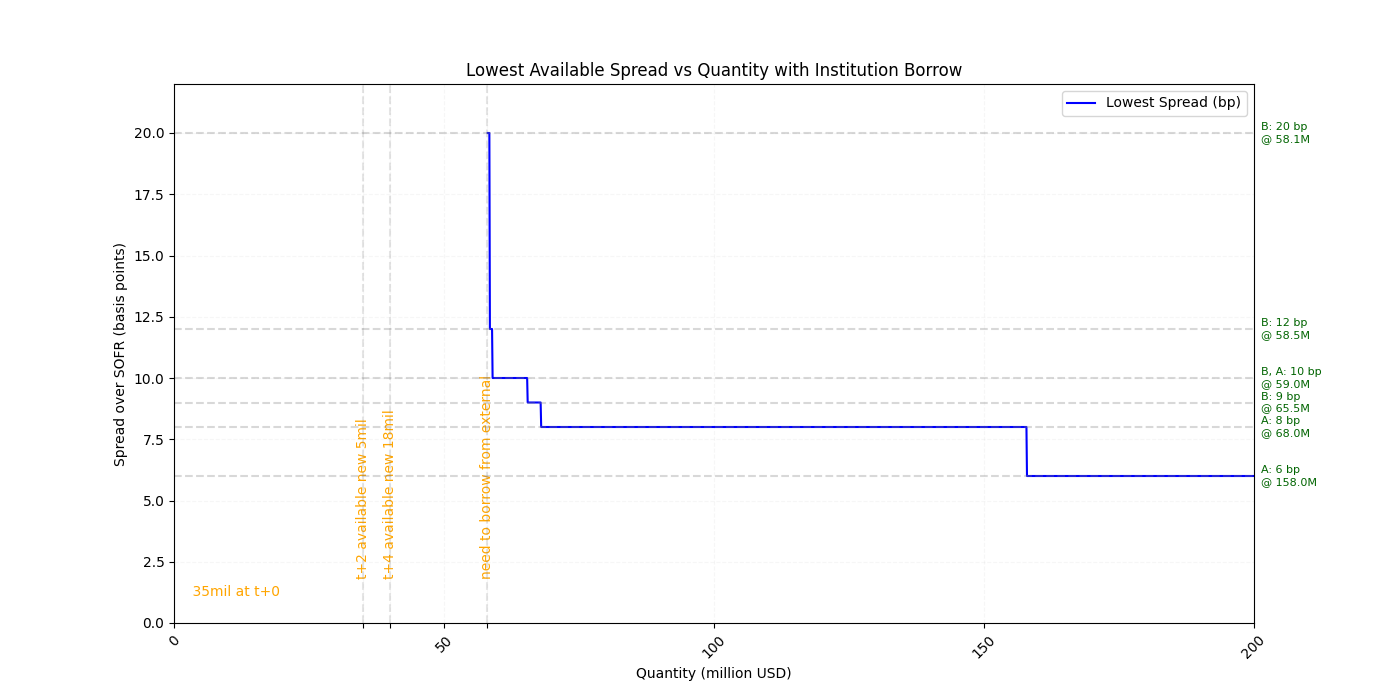
</br>
A REPO Trade End Cash Estimation Example
There is a REPO trade:
- Booked on 30-Jun-2024 (lent money out, received pledged security), first leg, bought $70,000,000$ units
- Expected second/end leg ended on 31-Aug-2025
- The pledged underlying security is a bond with ACT/360 and coupon rate $6.07\%$
- The REPO rate is bound to SOFR + 60 bp
- The start (dirty) price of bond is $100.94$
- The haircut is $10\%$
Business Explained:
- The rate bound to SOFR + 60 bp means that, SOFR is the U.S. interbank rate that can be regarded as risk-free cash cost, and the added 60 bp is the profit
- The haircut of $10\%$ means the value of the underlying security is discounted to $\times 90\%$ as the start cash lent to cash borrower; the discount of $10\%$ is risk margin in case the security value fluctuates
- The coupon rate of $6.07\%$ does NOT go into calculation for REPO rate does not see title transfer, coupon yield not transferred
Assume today is 15-Jul-2024, to compute end cash:
- Start Cash: $63,592,200 = 100.94 \times 70000000/100 \times 0.9$
- Compute REPO rate till today by SOFR (from 01-Jul-2024 to 15-Jul-2024), a total of 14 days since trade start date
| Date | SOFR (%) | SOFR (decimal) |
|---|---|---|
| 01-Jul-2024 | 5.4 | 0.054 |
| 02-Jul-2024 | 5.35 | 0.0535 |
| 03-Jul-2024 | 5.33 | 0.0533 |
| 05-Jul-2024 | 5.32 | 0.0532 |
| 08-Jul-2024 | 5.32 | 0.0532 |
| 09-Jul-2024 | 5.34 | 0.0534 |
| 10-Jul-2024 | 5.34 | 0.0534 |
| 11-Jul-2024 | 5.34 | 0.0534 |
| 12-Jul-2024 | 5.34 | 0.0534 |
| 15-Jul-2024 | 5.34 | 0.0534 |
By 360-day basis, compound rate is
\[\begin{align*} \text{TodayCompoundRate}_{14} &=1.0023116439864934 \\ &= \underbrace{\big(1+(0.054+0.006)/360\big)}_{\text{01-Jul-2024}} \times \underbrace{\big(1+(0.0535+0.006)/360\big)}_{\text{02-Jul-2024}} \times \underbrace{\big(1+(0.0533+0.006)/360\big)^{2}}_{\text{03-Jul-2024 to 04-Jul-2024}} \\ &\qquad \times \underbrace{\big(1+(0.0532+0.006)/360\big)^4}_{\text{05-Jul-2024 to 08-Jul-2024}} \times \underbrace{\big(1+(0.0534+0.006)/360\big)^6}_{\text{09-Jul-2024 to 14-Jul-2024}} \end{align*}\]Alternatively, if by linear rate, there is
\[\begin{align*} \text{TodayLinearRate}_{14} &=1.0023091666666668 \\ &= 1+ \underbrace{\big((0.054+0.006)/360\big)}_{\text{01-Jul-2024}} + \underbrace{\big((0.0535+0.006)/360\big)}_{\text{02-Jul-2024}} + \underbrace{\big((0.0533+0.006)/360 \times 2\big)}_{\text{03-Jul-2024 to 04-Jul-2024}} \\ &\qquad + \underbrace{\big((0.0532+0.006)/360 \times 4 \big)}_{\text{05-Jul-2024 to 08-Jul-2024}} + \underbrace{\big((0.0534+0.006)/360 \times 6\big)}_{\text{09-Jul-2024 to 14-Jul-2024}} \end{align*}\]- Use 5.34 for the all remaining days (the inferred SOFR rate can be derived using complex extrapolation methods as well, here used end static 5.34 for future date rate extrapolation). There are 412 days between 15-Jul-2024 and 31-Aug-2025.
- Final estimated end cash
- Also, the annualized rate is