Diffusion Model

September 12, 2025

Image data is added Gaussian noises multiple $T$ times (usually $T=500, 1000, 1500, 2000$) and eventually becomes absolute Gaussian noise. Diffusion model learns this behavior reversely so that the model knows how pixel should get updated by what patterns between two chronologically related image frames.

There are different ways to explain diffusion models, below uses Denoising Diffusion Probabilistic Models (DDPM)

References:

• https://zhuanlan.zhihu.com/p/525106459
• https://lilianweng.github.io/posts/2021-07-11-diffusion-models/

</br>

Diffusion Forward

Provided an image $\mathbf{x}_0\sim q(\mathbf{x})$, Gaussian noise is added to derive $\mathbf{x}_1, \mathbf{x}_2, …, \mathbf{x}_T$ image frames. This process is named $q$ process.

Let ${\beta_t \in (0,1)}^T_{t=1}$ be Gaussian variances. For each $t$ moment the forward is only related to the previous $t-1$ moment, the process is a Markov process:

\[\begin{align*} q(\mathbf{x}_t\|\mathbf{x}_{t-1}) &= \mathcal{N}(\mathbf{x}_t; \sqrt{1-\beta_t}\mathbf{x}_{t-1}, \beta_t\mathbf{I}) \\ q(\mathbf{x}_{1:T}\|\mathbf{x}_{0}) &= \prod^T_{i=1} q(\mathbf{x}_t\|\mathbf{x}_{t-1}) \end{align*}\]

Apparently, as $t$ increases, $\mathbf{x}_t$ approaches to pure Gaussian noise.

Reparameterization Trick

Differentiation in sampling from a distribution is not applicable. Reparameterization trick comes in help to make the process differentiable by an introduced independent variable $\epsilon$.

For example, to sample from a Gaussian distribution $z\sim \mathcal{N}(z;\mu_\theta, \sigma_\theta^2 I)$, it can be written as

\[z=\mu_\theta+\sigma_\theta \odot\epsilon,\quad \epsilon\sim \mathcal{N}(0,I)\]

where $\mu_\theta, \sigma_\theta$ are mean and variance of a Gaussian distribution that is determined by a neural network parameterized by $\theta$. The differentiation is on $\epsilon$.

Why Used ${1-\beta_t}$ as Variance in Progress

The primary role of $\beta_t$ is to control the variance, or amount, of Gaussian noise that is added to an image at each timestep t in the forward process. Then, define $\alpha_t = 1 - \beta_t$ that represents the proportion of the signal (the previous image $\mathbf{x}_{t-1 }$)that is preserved at each step.

While $\beta_t$ controls the noise, $\alpha_t$ controls how much of the original image’s characteristics are kept. A high $\alpha_t$ means less noise is added, and more of the signal is preserved.

Recall that $q(\mathbf{x})$ needs to maintain every $\mathbf{x}_t$ converge to $\mathcal{N}(0, I)$ for $t=1,2,…,T$. In any arbitrary step $t$, the progress can be expressed as

\[\begin{align*} \mathbf{x}_t &= \sqrt{\alpha_t}\mathbf{x}_{t-1}+\sqrt{1-\alpha_t}\space\mathbf{z}_{1} \\ &= \sqrt{\alpha_t}\left(\sqrt{\alpha_{t-1}}\mathbf{x}_{t-2}+\sqrt{1-\alpha_{t-1}}\mathbf{z}_{2}\right)+\sqrt{1-\alpha_t}\space\mathbf{z}_{1} \\ &= \sqrt{\alpha_t \alpha_{t-1}}\mathbf{x}_{t-2}+\left(\sqrt{\alpha_t}\sqrt{1-\alpha_{t-1}}\mathbf{z}_{2}+\sqrt{1-\alpha_t}\space\mathbf{z}_{1} \right) \\ &= \sqrt{\alpha_t \alpha_{t-1} \alpha_{t-2}}\mathbf{x}_{t-3}+\left(\sqrt{\alpha_{t-1}}\sqrt{1-\alpha_{t-2}}\mathbf{z}_{3}+\sqrt{\alpha_t}\sqrt{1-\alpha_{t-1}}\mathbf{z}_{2}+\sqrt{1-\alpha_t}\space\mathbf{z}_{1} \right) \\ &= ... \\ \end{align*}\]

where $\mathbf{z}{1}, \mathbf{z}{2}, … \sim \mathcal{N}(0,I)$.

Given the sum property of Gaussian distribution independence, there is $\mathcal{N}(0,\sigma_1^2 I)+\mathcal{N}(0,\sigma_2^2 I)\sim \mathcal{N}\left(0,(\sigma_1^2+\sigma_2^2)I\right)$, so that

\[\begin{align*} \sqrt{\alpha_{t}}\sqrt{1-\alpha_{t-1}}\mathbf{z}_{2}+\sqrt{1-\alpha_t}\space\mathbf{z}_{1} &\sim \mathcal{N}\left(0, ({\alpha_{t}}({1-\alpha_{t-1}})+{1-\alpha_t})I\right) \\ &= \mathcal{N}\left(0, (1-\alpha_t\alpha_{t-1})I\right) \\ \end{align*}\]

Let $\overline{\alpha}t=\prod^t{\tau=1}\alpha_{\tau}$ be the chained product, the above $\mathbf{x}_t$ can be expressed as

\[\begin{align*} \mathbf{x}_t &= \sqrt{\alpha_t \alpha_{t-1} \alpha_{t-2}}\mathbf{x}_{t-3}+\left(\sqrt{\alpha_{t-1}}\sqrt{1-\alpha_{t-2}}\mathbf{z}_{3}+\sqrt{\alpha_t}\sqrt{1-\alpha_{t-1}}\mathbf{z}_{2}+\sqrt{1-\alpha_t}\space\mathbf{z}_{1} \right) \\ &= \sqrt{\alpha_t \alpha_{t-1} \alpha_{t-2}}\mathbf{x}_{t-3}+ \left(\sqrt{1-{\alpha}_{t}{\alpha}_{t-1}{\alpha}_{t-2}}\space\overline{\mathbf{z}}_{1:3}\right)\\ &= ... \\ &= \sqrt{\overline{\alpha}_t}\space\mathbf{x}_{0}+\sqrt{1-\overline{\alpha}_t}\space\overline{\mathbf{z}_{t}} \end{align*}\]

Choices of $\alpha_t$ and $\beta_t$

• Linear Schedule

Formula: $\beta_t$ goes from $\beta_{start} = 0.0001$ to $\beta_{start} = 0.002$ over $T$ timesteps (e.g., $T=1000$).

• Cosine Schedule

Formula: It’s defined based on the cumulative $\overline{\alpha}_t$, following a cosine function shape.

The schedule is much more gradual. $\beta_t$ starts extremely small and increases very slowly, preventing the model from losing information too quickly.

The rate of noise addition then speeds up through the middle of the process before slowing down again at the very end.

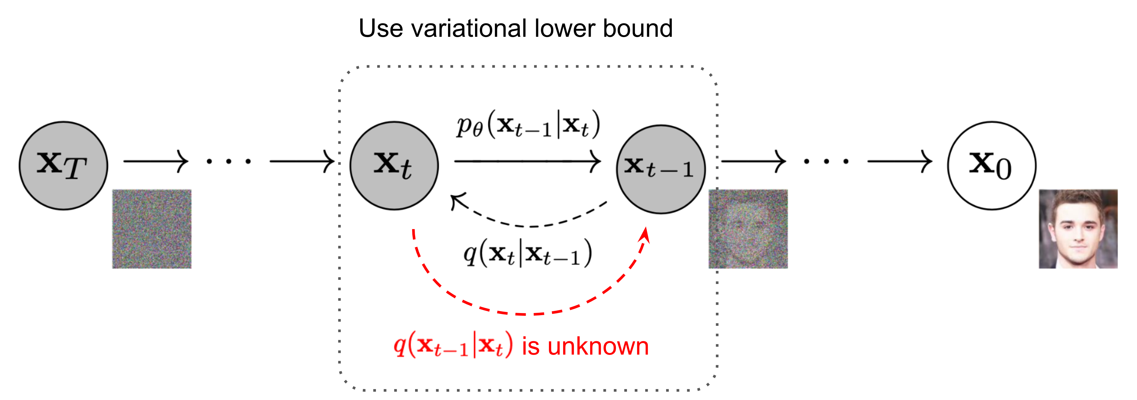
Reverse Diffusion Process

The reverse process is to remove noise such that by iterative step $q(\mathbf{x}{t-1}|\mathbf{x}{t})$ the source image $\mathbf{x}{0}$ can be derived from pure Gaussian noise $\mathbf{x}{T}\sim \mathcal{N}(0, I)$.

</br>

$q(\mathbf{x}{t-1}|\mathbf{x}{t})$ is difficult to learn. This is for that noises can be added by a known sequence of steps $\mathbf{z}{1}, \mathbf{z}{2}, … \sim \mathcal{N}(0,I)$ added to $\mathbf{x}{t-1}$ to derive $\mathbf{x}{t}$, but noise removal from $\mathbf{x}_{t}$ is very difficult.

The philosophy can be explained by the scenario that provided a large dataset, it is easy to place a random wronged sample in the dataset (forward process), but to find out the wronged sample (reverse process), unless already known the error placement scheme, it needs to traverse the entire dataset to locate the wronged sample.

In other words, given a noisy image $\mathbf{x}{t}$, it is unknown for each pixel by what values (e.g., RGB) to adjust so that $\mathbf{x}{t}$ can find the exact pixel match of $\mathbf{x}{t-1}$. For an image sized $480 \times 480$ by 8-bit RGB encoding, it takes $480 \times 480 \times 256 \times 3$ pixel change attempts to find out which one pixel combination and permutation scenario matches against that of $\mathbf{x}{t-1}$.

The reverse process $q(\mathbf{x}{t-1}|\mathbf{x}{t})$ is very computation-intensive unless the noise addition pattern is known.

Bayes’ Rule Trick for Reverse Diffusion Process

As explained above, $q(\mathbf{x}{t-1}|\mathbf{x}{t})$ would be extremely expensive in computation for it needs to exhaust all combination and permutation scenarios to find $\mathbf{x}{t-1}$. However, if provided original image $\mathbf{x}{0}$, the learning can fast converge without exhaustion.

\[q(\mathbf{x}_{t-1}\|\mathbf{x}_{t},\mathbf{x}_{0})= \mathcal{N}\big(\mathbf{x}_{t-1};\tilde{\mu}_\theta(\mathbf{x}_{t},\mathbf{x}_{0}),\tilde{\beta}_t I\big)\]

Below proves how to leverage $\mathbf{x}{0}$ and $\mathbf{x}{t}$ to compute $\mathbf{x}_{t-1}$ by Bayes’ rule to make the reverse process a forward one. A forward process is known a Gaussian noise addition.

By Bayes’ rule, conditioned on original image $\mathbf{x}_{0}$, there is

\[q(\mathbf{x}_{t-1}\|\mathbf{x}_{t},\mathbf{x}_{0})= q(\mathbf{x}_{t}\|\mathbf{x}_{t-1},\mathbf{x}_{0})\frac{q(\mathbf{x}_{t-1}\|\mathbf{x}_{0})}{q(\mathbf{x}_{t}\|\mathbf{x}_{0})}\]

where in the Bayes’ rule expression all expressions are of forward such that $(\mathbf{x}{t-1},\mathbf{x}{0}) \rightarrow \mathbf{x}{t}$, $\mathbf{x}{t-1} \rightarrow \mathbf{x}{t}$ and $\mathbf{x}{0} \rightarrow \mathbf{x}_{t}$.

Recall that noise $\mathbf{z}t$ is derived from a Gaussian distribution and the propagation is $\mathbf{x}_t=\sqrt{\alpha_t}\mathbf{x}{t-1}+\sqrt{1-\alpha_t}\space\mathbf{z}_t$.

\[\begin{align*} && \mathbf{x}_t &=\sqrt{\alpha_t}\mathbf{x}_{t-1}+\sqrt{1-\alpha_t}\space\mathbf{z}_t \\ && &= \sqrt{\alpha_t}\mathbf{x}_{t-1}+\sqrt{\beta_t}\space\mathbf{z}_t & \text{where } \mathbf{z}_t\sim \mathcal{N}(0,I) \end{align*}\]

In other words, $\mathbf{x}t$ takes $\sqrt{\alpha_t}\mathbf{x}{t-1}$ as mean with added noise $\sqrt{\beta_t}\space\mathbf{z}_t$.

By the definition $X\sim \mathcal{N}(\mu, \sigma^2)$ as $f(x)=\frac{1}{\sigma\sqrt{2\pi}}\exp(-\frac{(x-\mu)^2}{2\sigma^2})$, the Gaussian density distribution for the forward process is $q(\mathbf{x}{t}|\mathbf{x}{t-1})\propto\exp\Big(-\frac{(\mathbf{x}t-\sqrt{\alpha_t}\mathbf{x}{t-1})^2}{2\beta_t}\Big)$.

Similarly, there are $q(\mathbf{x}{t-1}|\mathbf{x}{0})\propto\exp\Big(-\frac{(\mathbf{x}t-\sqrt{\overline{\alpha}{t-1}}\mathbf{x}{0})^2}{2(1-\overline{\alpha}{t-1})}\Big)$ and $q(\mathbf{x}{t}|\mathbf{x}{0})\propto\exp\Big(-\frac{(\mathbf{x}t-\sqrt{\overline{\alpha}{t}}\mathbf{x}{0})^2}{2(1-\overline{\alpha}{t})}\Big)$.

As a result, the reverse process can be rewritten as

\[\begin{align*} q(\mathbf{x}_{t-1}\|\mathbf{x}_{t},\mathbf{x}_{0})&= q(\mathbf{x}_{t}\|\mathbf{x}_{t-1},\mathbf{x}_{0})\frac{q(\mathbf{x}_{t-1}\|\mathbf{x}_{0})}{q(\mathbf{x}_{t}\|\mathbf{x}_{0})} \\ &\propto \exp\left(-\frac{1}{2}\left(\frac{(\mathbf{x}_t-\sqrt{\alpha_t}\mathbf{x}_{t-1})^2}{\beta_t}+ \frac{(\mathbf{x}_t-\sqrt{\overline{\alpha}_{t-1}}\mathbf{x}_{0})^2}{1-\overline{\alpha}_{t-1}}- \frac{(\mathbf{x}_t-\sqrt{\overline{\alpha}_{t}}\mathbf{x}_{0})^2}{1-\overline{\alpha}_{t}}\right)\right) \\ &= \exp\left(-\frac{1}{2} \left( \left(\frac{\alpha_t}{\beta_t} + \frac{1}{1-\bar{\alpha}_{t-1}}\right)\mathbf{x}_{t-1}^2 - \left(\frac{2\sqrt{\alpha_t}}{\beta_t}\mathbf{x}_t + \frac{2\sqrt{\bar{\alpha}_{t-1}}}{1-\bar{\alpha}_{t-1}}\mathbf{x}_0\right)\mathbf{x}_{t-1} + C(\mathbf{x}_t, \mathbf{x}_0) \right) \right) \end{align*}\]

where for any general Gaussian density function there is $\exp(-\frac{(x-\mu)^2}{2\sigma^2})=\exp\big(-\frac{1}{2}(\frac{1}{\sigma^2}x^2-\frac{2\mu}{\sigma^2}x+\frac{\mu^2}{\sigma^2})\big)$, the mean and variance of $q(\mathbf{x}{t-1}|\mathbf{x}{t},\mathbf{x}_{0})$ can be derived from coefficient mapping.

The variance is

\[\begin{align*} && \frac{1}{\sigma^2} &= \left(\frac{\alpha_t}{\beta_t} + \frac{1}{1-\bar{\alpha}_{t-1}}\right) \\ \Rightarrow && \tilde{\beta}_t &= 1 / \left(\frac{\alpha_t}{\beta_t} + \frac{1}{1-\bar{\alpha}_{t-1}}\right) = 1/ \left(\frac{1-\beta_t}{\beta_t} + \frac{1}{1-\bar{\alpha}_{t-1}}\right) = \frac{1-\bar{\alpha}_{t-1}}{1-\bar{\alpha}_t} \beta_t \end{align*}\]

The mean is

\[\begin{align*} && \frac{2\mu}{\sigma^2} &= \left(\frac{2\sqrt{\alpha_t}}{\beta_t}\mathbf{x}_t + \frac{2\sqrt{\bar{\alpha}_{t-1}}}{1-\bar{\alpha}_{t-1}}\mathbf{x}_0\right) \\ \Rightarrow && \tilde{\mathbf{\mu}}_t(\mathbf{x}_t, \mathbf{x}_0) &= \left(\frac{\sqrt{\alpha_t}}{\beta_t}\mathbf{x}_t + \frac{\sqrt{\bar{\alpha}_{t-1}}}{1-\bar{\alpha}_{t-1}}\mathbf{x}_0\right) \tilde{\beta}_t = \frac{\sqrt{\alpha_t}(1-\bar{\alpha}_{t-1})}{1-\bar{\alpha}_t} \mathbf{x}_t + \frac{\sqrt{\bar{\alpha}_{t-1}}\beta_t}{1-\bar{\alpha}_t} \mathbf{x}_0 \end{align*}\]

Given previously already proved $\mathbf{x}t = \sqrt{\overline{\alpha}_t}\space\mathbf{x}{0}+\sqrt{1-\overline{\alpha}t}\space\overline{\mathbf{z}{t}}$ that gives $\mathbf{x}{0} = \frac{1}{\sqrt{\overline{\alpha}_t}}\big(\mathbf{x}_t-\sqrt{1-\overline{\alpha}_t}\space\overline{\mathbf{z}{t}}\big)$, replace $\mathbf{x}_0$ with an expression of $\mathbf{x}_t$ in $\tilde{\mathbf{\mu}}_t(\mathbf{x}_t, \mathbf{x}_0)$ to remove the irrelevant $\mathbf{x}_0$ so that $\tilde{\mathbf{\mu}}$ is just a function of $\mathbf{x}_t$:

\[\tilde{\mathbf{\mu}}_t(\mathbf{x}_t) = \frac{1}{\sqrt{\alpha_t}} \left( \mathbf{x}_t - \frac{\beta_t}{\sqrt{1 - \bar{\alpha}_t}} \space\overline{\mathbf{z}}_t \right)\]

where $\overline{\mathbf{z}}t$ is the model $\theta$ predicted noise, rewrite it to $\mathbf{z}{\theta}(\mathbf{x}_t, t)$.

\[\mathbf{\mu}_{\theta}(\mathbf{x}_t, t) = \frac{1}{\sqrt{\alpha_t}} \left( \mathbf{x}_t - \frac{\beta_t}{\sqrt{1 - \bar{\alpha}_t}} \space\mathbf{z}_{\theta}(\mathbf{x}_t, t) \right)\]

Reverse Process Step Summary

Within the whole process:

1. At each step $t$ compute $\mathbf{\mu}_{\theta}(\mathbf{x}_t, t)$.
2. Given small noise propagation $\overline{\alpha}t\approx\overline{\alpha}{t-1}$, it can be said $\tilde{\beta}t=\frac{1-\bar{\alpha}{t-1}}{1-\bar{\alpha}_t}\beta_t\approx\beta_t$

Diffusion Training

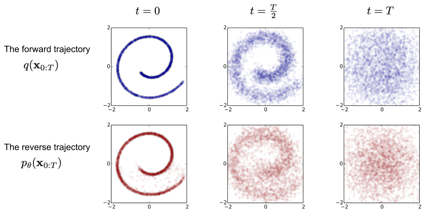
Let $p_{\theta}(\mathbf{x}_{0:T})$ be the reverse diffusion process probability, there are

\[\begin{align*} p_{\theta}(\mathbf{x}_{0:T})&=p(\mathbf{x}_{T})\prod^T_{t=1}p_\theta(\mathbf{x}_{t-1}\|\mathbf{x}_{t}) \\ p_{\theta}(\mathbf{x}_{t-1}\|\mathbf{x}_{t})&=\mathcal{N}\big(\mathbf{x}_{t-1};\mu_\theta(\mathbf{x}_{t},t),\Sigma_\theta(\mathbf{x}_{t},t)\big) \\ \end{align*}\]

This chapter explains how to train a diffusion model to derive at eact time $t$ the optimal ${\mathbf{\mu}}{\theta}(\mathbf{x}_t, t)$ and ${\mathbf{\Sigma}}{\theta}(\mathbf{x}t, t)$ with assumed $\mathbf{x}_0\sim q(\mathbf{x}_0)$ by minimizing cross-entropy of $p{\theta}(\mathbf{x}_{0})$.

In other words, to maximize $p_{\theta}(\mathbf{x}_{0:T})$, it is equivalent to

\[\begin{align*} && \max\int \dots \int \int p_\theta(\mathbf{x}_0, \mathbf{x}_1, \dots, \mathbf{x}_T) \; d\mathbf{x}_1 d\mathbf{x}_2 \dots d\mathbf{x}_T &=\int p_\theta(\mathbf{x}_{0:T}) d\mathbf{x}_{1:T} \\ \Rightarrow && \min\mathcal{L}_{\text{CE}} &=\mathbb{E}_{q(\mathbf{x}_{0})}\big(-\log p_{\theta}(\mathbf{x}_{0})\big) \end{align*}\]

This chapter will later reveal that diffusion training is essentially to minimize the MSE between $\overline{\mathbf{z}{t}}$ vs $\mathbf{z}{\theta}$ so that model $\theta$ knows gradual pixel change to approximate the source image $\mathbf{x}_{0}$.

$p_\theta(\mathbf{x}0)$ is the marginal probability of the data $\mathbf{x}_0$, while $p\theta(\mathbf{x}_{0:T})$ is the joint probability of the entire sequence of variables from $\mathbf{x}_0$ to $\mathbf{x}_t$.

\[\begin{align*} \mathcal{L}_{\text{CE}} &= - \mathbb{E}_{q(\mathbf{x}_0)} \log p_\theta(\mathbf{x}_0) \\ &= - \mathbb{E}_{q(\mathbf{x}_0)} \log \left( \int p_\theta(\mathbf{x}_{0:T}) d\mathbf{x}_{1:T} \right) \\ &= - \mathbb{E}_{q(\mathbf{x}_0)} \log \left( \int q(\mathbf{x}_{1:T} \| \mathbf{x}_0) \frac{p_\theta(\mathbf{x}_{0:T})}{q(\mathbf{x}_{1:T} \| \mathbf{x}_0)} d\mathbf{x}_{1:T} \right) \\ &= - \mathbb{E}_{q(\mathbf{x}_0)} \log \left( \mathbb{E}_{q(\mathbf{x}_{1:T} \| \mathbf{x}_0)} \frac{p_\theta(\mathbf{x}_{0:T})}{q(\mathbf{x}_{1:T} \| \mathbf{x}_0)} \right) \\ &\leq - \mathbb{E}_{q(\mathbf{x}_{0:T})} \log \frac{p_\theta(\mathbf{x}_{0:T})}{q(\mathbf{x}_{1:T} \| \mathbf{x}_0)} &\text{Jensen's Inequality} \\ &= \mathbb{E}_{q(\mathbf{x}_{0:T})} \left[ \log \frac{q(\mathbf{x}_{1:T} \| \mathbf{x}_0)}{p_\theta(\mathbf{x}_{0:T})} \right] \\ &= \mathcal{L}_{\text{VLB}} \end{align*}\]

To convert each term in the equation to be analytically computable, the objective can be further rewritten to be a combination of several KL-divergence and entropy terms.

\[\begin{align*} \mathcal{L}_{\text{VLB}} &= \mathbb{E}_{q(\mathbf{x}_{0:T})} \left[ \log \frac{q(\mathbf{x}_{1:T} \| \mathbf{x}_0)}{p_\theta(\mathbf{x}_{0:T})} \right] \\ &= \mathbb{E}_q \left[ \log \frac{\prod_{t=1}^T q(\mathbf{x}_t\|\mathbf{x}_{t-1})}{p_\theta(\mathbf{x}_T) \prod_{t=1}^T p_\theta(\mathbf{x}_{t-1}\|\mathbf{x}_t)} \right] \\ &= \mathbb{E}_q \left[ -\log p_\theta(\mathbf{x}_T) + \sum_{t=1}^T \log \frac{q(\mathbf{x}_t\|\mathbf{x}_{t-1})}{p_\theta(\mathbf{x}_{t-1}\|\mathbf{x}_t)} \right] \\ &= \mathbb{E}_q \left[ -\log p_\theta(\mathbf{x}_T) + \sum_{t=2}^T \log \frac{q(\mathbf{x}_{t-1}\|\mathbf{x}_t, \mathbf{x}_0)}{p_\theta(\mathbf{x}_{t-1}\|\mathbf{x}_t)} \cdot \frac{q(\mathbf{x}_t\|\mathbf{x}_0)}{q(\mathbf{x}_{t-1}\|\mathbf{x}_0)} + \log \frac{q(\mathbf{x}_1\|\mathbf{x}_0)}{p_\theta(\mathbf{x}_0\|\mathbf{x}_1)} \right] \\ &= \mathbb{E}_q \left[ \underbrace{D_{\text{KL}}(q(\mathbf{x}_T\|\mathbf{x}_0) \|\| p_\theta(\mathbf{x}_T))}_{\mathcal{L}_{\text{T}}} + \sum_{t=2}^T \underbrace{D_{\text{KL}}(q(\mathbf{x}_{t-1}\|\mathbf{x}_t, \mathbf{x}_0) \|\| p_\theta(\mathbf{x}_{t-1}\|\mathbf{x}_t))}_{\mathcal{L}_{\text{t-1}}} - \underbrace{\log p_\theta(\mathbf{x}_0\|\mathbf{x}_1)}_{\mathcal{L}_{\text{0}}} \right] \\ &= \mathcal{L}_{\text{T}} + \mathcal{L}_{\text{T-1}} + \mathcal{L}_{\text{T-2}} + ... + \mathcal{L}_{\text{0}} \end{align*}\]

where $\mathcal{L}{\text{T}}$ and $\mathcal{L}{\text{0}}$ are constant hence ignorable for $\mathbf{x}_T$ and $\mathbf{x}_0$ are constant.

For each $\mathcal{L}{\text{t}}$, $p\theta(\mathbf{x}{t-1}|\mathbf{x}_t)$ should approximate $q(\mathbf{x}{t-1}|\mathbf{x}_t, \mathbf{x}_0)$:

\[\begin{align*} q(\mathbf{x}_{t-1}\|\mathbf{x}_t, \mathbf{x}_0) &=\mathcal{N}\left(\mathbf{x}_{t-1};\tilde{\mathbf{\mu}}_t(\mathbf{x}_t, \mathbf{x}_0), \tilde{\beta}_t I\right) \\ p_\theta(\mathbf{x}_{t-1}\|\mathbf{x}_t) &=\mathcal{N}\left(\mathbf{x}_{t-1};{\mathbf{\mu}}_t(\mathbf{x}_t, \mathbf{x}_0), \Sigma_\theta\right) \end{align*}\]

By the definition of the relative entropy (Kullback-Leibler divergence) between two multivariate ($k$-dimension) normal distributions $\mathcal{N}_0(\mu_0,\Sigma_0)$ and $\mathcal{N}_1(\mu_1,\Sigma_1)$ is as below

\[D_{\text{KL}}(\mathcal{N}_0 \\| \mathcal{N}_1) = \frac{1}{2} \left( \operatorname{tr}(\Sigma_1^{-1}\Sigma_0) + (\mu_1 - \mu_0)^T \Sigma_1^{-1} (\mu_1 - \mu_0) - k + \ln\left(\frac{\det(\Sigma_1)}{\det(\Sigma_0)}\right) \right)\]

Although $\Sigma_\theta$ is also learnable to align to $\tilde{\beta}t I$, the naive approach adopted in this chapter only considers learning $\mu\theta$ for explanation purposes. Here writes $\mathcal{L}_{\text{t}}$ to

\[\mathcal{L}_{\text{t}} = E_q \left[ \frac{1}{2\|\|\Sigma_\theta(\mathbf{x}_t,t)\|\|_2^2} \Big\|\Big\| \tilde{\mu}_t(\mathbf{x}_t, x_0) - \mu_\theta(\mathbf{x}_t, t) \Big\|\Big\|^2 \right] + C\]

where $C$ is a constance to represent irrelevant $\Sigma_\theta$ to $\tilde{\beta}_t I$.

In other words, $\mathcal{L}{\text{t}}$ is essential the L2 distance between the two normal distribution means $\tilde{\mu}_t(\mathbf{x}_t, x_0)$ vs $\mu\theta(\mathbf{x}_t, t)$.

The actual model $\theta$ prediction should be the approximated noises $\mathbf{z}{\theta}$. Here convert the expression back to using $\mathbf{z}{\theta}$.

\[\begin{align*} \mathcal{L}_{\text{t}} &= E_q \left[ \frac{1}{2\|\|\Sigma_\theta(\mathbf{x}_t,t)\|\|_2^2} \Big\|\Big\| \tilde{\mu}_t(\mathbf{x}_t, x_0) - \mu_\theta(\mathbf{x}_t, t) \Big\|\Big\|^2 \right] \\ &= \mathbb{E}_{\mathbf{x}_0, \mathbf{z}} \left[ \frac{1}{2 \\| \Sigma_\theta \\|_2^2} \left\\| \frac{1}{\sqrt{\alpha_t}} \left( \mathbf{x}_t - \frac{1 - \alpha_t}{\sqrt{1 - \bar{\alpha}_t}} \mathbf{z}_t \right) - \frac{1}{\sqrt{\alpha_t}} \left( \mathbf{x}_t - \frac{1 - \alpha_t}{\sqrt{1 - \bar{\alpha}_t}} \mathbf{z}_\theta(\mathbf{x}_t, t) \right) \right\\|^2 \right] \\ &= \mathbb{E}_{\mathbf{x}_0, \mathbf{z}} \left[ \frac{(1 - \alpha_t)^2}{2 \alpha_t (1 - \bar{\alpha}_t) \\| \Sigma_\theta \\|_2^2} \\| \mathbf{z}_t - \mathbf{z}_\theta(\sqrt{\bar{\alpha}_t}\mathbf{x}_0 + \sqrt{1 - \bar{\alpha}_t}\mathbf{z}_t, t) \\|^2 \right] \end{align*}\]

Finally, the result reveals the loss $\mathcal{L}{\text{t}}$ how it is influenced by model output $\mathbf{z}{\theta}$.