embedding and rope
February 05, 2025
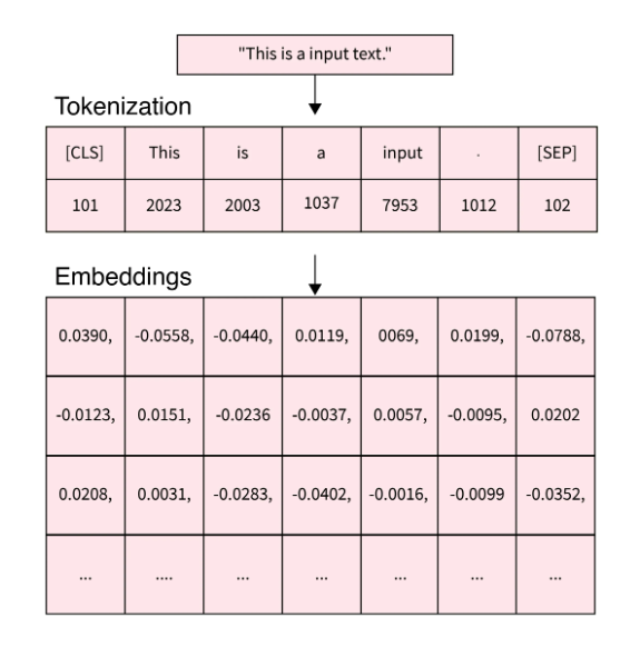
Embedding describes information representation and compression, representing a token/word as a vector.
</br>
Semantics/Linguistics
For example, the word “restaurants” has the below attributes:
- isNoun: ${0, 0, 0, 1, 0}$ for ${\text{isVerb}, \text{isAdjective}, \text{isPronoun}, \text{isNoun}, \text{isAdverb}}$
- isPlural: ${1}$ for ${\text{isPlural}}$
- synonyms: ${ 5623, 1850, 2639 }$ (vocabulary index) for ${ \text{hotel}, \text{bar}, \text{club} }$
- antonyms: $\emptyset$
- frequent occurrences under what topics: ${ 1203, 5358, 1276 }$ (vocabulary index) for ${ \text{eating}, \text{outing}, \text{gathering} }$
- Term frequency-inverse document frequency (TF-IDF): ${ 0.016, 0.01, 0.0, 0.005 }$ , formula:
- \(\text{TF-IDF}_j = \text{Term Frequency}_{i,j} \times \text{Inverse Document Frequency}_{i}\), where
- $\text{Term Frequency}_{i,j} = \frac{\text{Term i frequency in document j}}{\text{Total no. of terms in document j}}$
- $\text{Inverse Document Frequency}_{i} = \log \frac{\text{Total no. of documents}}{\text{No. of documents containing term i}}$
Given the four sentences/documents,
There are many popular restaurants nearby this church.
Some restaurants offer breakfasts as early as 6:00 am to provide for prayers.
"The price and taste are all good.", said one prayer who has been a frequent visitor to this church since 1998.
However, Covid-19 has forced some restaurants to shut down for lack of revenue during the pandemic, and many prayers are complained about it.
The TF-IDF per sentence/document is computed as below.
| No. | Token | Term count (Doc 1) | Term count (Doc 2) | Term count (Doc 3) | Term count (Doc 4) | Document count | IDF | TF $\times$ IDF (Doc 1) | TF $\times$ IDF (Doc 2) | TF $\times$ IDF (Doc 3) | TF $\times$ IDF (Doc 4) |
|---|---|---|---|---|---|---|---|---|---|---|---|
| 1 | many | 0.125 | 0 | 0 | 0.04348 | 2 | 0.301 | 0.038 | 0 | 0 | 0.013 |
| 2 | popular | 0.125 | 0 | 0 | 0 | 1 | 0.602 | 0.075 | 0 | 0 | 0 |
| 3 | restaurants | 0.125 | 0.07692 | 0 | 0.04348 | 3 | 0.125 | 0.016 | 0.01 | 0 | 0.005 |
| 4 | nearby | 0.125 | 0 | 0 | 0 | 1 | 0.602 | 0.075 | 0 | 0 | 0 |
| 5 | church | 0.125 | 0 | 0.04762 | 0 | 2 | 0.301 | 0.038 | 0 | 0.014 | 0 |
| 6 | offer | 0 | 0.07692 | 0 | 0 | 1 | 0.602 | 0 | 0.046 | 0 | 0 |
For compression, one popular approach is encoder/decoder, where dataset is fed to machine learning study.
For example, by placing “restaurants” and “bar” together in a text dataset that only describes food, likely the attribute “topic” might have little information hence neglected (set to zeros) in embeddings.
Rotational Position Embeddings (RoPE)
https://zhuanlan.zhihu.com/p/662790439
Positional embeddings represent the position of a word in a sentence/document. The order of how vocabularies are arranged in a sentence/document provides rich information in NLP.
Transformer uses the below formulas to compute positional embeddings (PE) by a rotation matrix $R(\bold{\theta}_i)$ where each token position is represented/offset by $\bold{\theta}_i$ with respect to dimension $\bold{i}$.
\[\begin{align*} \text{PE}(i) &= R (\bold{\theta}_i) \qquad \text{where } \bold{\theta}_i = 10000^{-\frac{2i}{\bold{D}}} \end{align*}\]where $\bold{i}={ 1,2,…,D } \in \mathbb{Z}^{+}$ is a vector of dimension indices, then define $\bold{\theta}_i=10000^{-\frac{2i}{\bold{D}}}$.
Intuition of Embedding Design Philosophy: Semantics Indicated By Dimensionality Encapsulated Token Distance Info
For a query token $\bold{q}_m\in\mathbb{R}^{1\times D}$ positioned at $m$ and a key token $\bold{k}_n\in\mathbb{R}^{1\times D}$ at $n$, and assume their respective dimensions correlate to the two token distance $|n-m|$ (corresponding frequency denoted as $\frac{1}{|n-m|}$, also distance is termed wavelength), by learning their embeddings encapsulates latent relationship.
- High frequency features: Detailed, rapid changes in position for local context.
- Low frequency features: Smooth, gradual changes that encode global structure in a long article.
| Besides, as two token distance grows $ | n-m | \rightarrow\infty$, from the perspective of human linguistics the two tokens should gradually lose latent connection, and token embeddings should reflect such linguistic phenomenon. |
Example To Explain High/Low Frequency Features: An Article About Pets
Below is an article discussing pets’ role in human society, and the article uses cats and dogs as examples for comparison for explanation.
Pets are considered global features, and cats and dogs are local.
Pets have long been cherished companions, bringing joy, comfort, and a sense of purpose into their owners' lives.

... (Some introduction and background)

Cats were domesticated around 9,000 years ago, likely drawn to human settlements for food, and were later adopted as pets for their hunting skills and companionship.

Dogs, domesticated over 15,000 years ago from wolves, were gradually adopted as pets due to their loyalty, ability to assist in hunting, and role as protectors of human communities.

Cats are admired for their independent yet affectionate nature. They bring a soothing presence into a home, often offering quiet moments of comfort and playful antics that lighten the mood.

Dogs, on the other hand, are renowned for their loyalty and exuberant spirit. They often act as the heartbeat of a household, encouraging physical activity and social interaction.

... (Some discussions on pet's engagement in human society)

As society continues to evolve, so does the landscape of pet ownership.
Advances in veterinary care, pet nutrition, and animal welfare are shaping a future where pets can lead longer, healthier lives.
In summary, pets play an indispensable role in enriching our lives through their companionship and unique traits.
Let \(\bold{q}_{\text{dogs}}\) be a query to see the latent relationship with a local concept \(\bold{k}_{\text{cats}}\) and a global one \(\bold{k}_{\text{pets}}\).
Let \(|n_{\text{dogs}}-m_{\text{cats}}|=\Delta_{50}=50\) represent “dogs” sees “cats” with a token distance of $50$, and let $|n_{\text{dogs}}-m_{\text{pets}}|=\Delta_{300}=300$ represent “dogs” sees “pets” with a token distance of $300$.
Let $\bold{freqDimTrans}(\Delta)\in\mathbb{R}^{1\times 1000}$ be the transform that maps a token embedding to distance-aware ones so that each dimension represents certain distance (this transform as an example covers $1k$ token length). It takes positional gap $\Delta$ as argument.
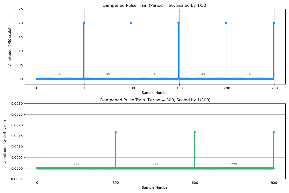
The dimensionality of the embedding indicates the distance info. Let \(\Pi(t)=\begin{cases} 1 & \quad t=1 \\ 0 & \quad \text{otherwise}\end{cases}\) be a pulse function that $\Pi(t)=1$ if and only if the input is a unit signal at $t=1$. Let $\bold{w}=[w_1, w_2, …, w_{1000}]$ be the weight coefficients, usually it sees a monotonic decaying progress as $w_i\rightarrow w_{1000}$, e.g., $w_i=1/{\Delta_{i}}$ is set up as reciprocal function.
\[\begin{align*} \bold{freqDimTrans}(\Delta)=\bigg[ & w_{1}\Pi(\frac{1}{1}\Delta), w_{2}\Pi(\frac{1}{2}\Delta), ..., w_{50}\Pi(\frac{1}{50}\Delta), ..., w_{300}\Pi(\frac{1}{300}\Delta), ..., w_{1000}\Pi(\frac{1}{1000}\Delta), \bigg] \end{align*}\]- $\Pi(\frac{1}{50}\Delta_{\text{dogs-cats}})$ should see weighted peaks at an interval of $50$.
- $\Pi(\frac{1}{300}\Delta_{\text{dogs-pets}})$ should see peaks at an interval of $300$.
</br>
For $300>50$ that long distance tokens should see each other less semantics, e.g., by $w_i=1/{\Delta_{i}}$, the peaks in this dimension are dampened to lower values.
Apply $\bold{freqDimTrans}(\Delta)$ to “dogs”, “cats”, and “pets”, only certain frequencies are fired up thereby having learned distance info.
RoPE Frequency Resonation Intuition
Instead of using a naive pulse signal, RoPE uses many rotation matrices to represent frequencies, where each dimension pair is set up to rotate by an angle $\Delta\theta_i$, and such angles have different resolution for different dimensions.
Let $R(\theta)$ be a rotation matrix
\[R (\theta_i) = \begin{bmatrix} \cos \theta_i & -\sin \theta_i \\ \sin \theta_i & \cos \theta_i \\ \end{bmatrix}, \qquad i=0,1,...,D/2-1\]Group dimensions by pairs for each rotation by $R (\theta_i)$ works on a 2-dimensional vector.
\[\begin{align*} \bold{q}&=\big[(q_1, q_2), (q_3, q_4), ..., (q_{D-1}, q_{D})\big] \\ \bold{k}&=\big[(k_1, k_2), (k_3, k_4), ..., (k_{D-1}, k_{D})\big] \\ \end{align*}\]The similarity (inverse correlation to distance) is measured by below.
\[\text{similarity}_{\cos}(\bold{q}_{i,i+1}, \bold{k}_{i,i+1}) = \cos(\Delta\theta_i) = \frac{\bold{q}_{i,i+1} \cdot \bold{k}_{i,i+1}}{||\bold{q}_{i,i+1} || \space || \bold{k}_{i,i+1} ||}\]When they are overlapping each other on particular dimensions, e.g., $\max_{\Delta\theta_i=0}=\cos(\Delta\theta_i)=1$ they resonate on the $i$-th dimension mapped token distance/frequency.
RoPE Derivation
Linear Position Embedding
Define a score to be maximized when query $\bold{q}_m$ is positionally “close” to key $\bold{k}_n$. The $i$ and $j$ individually represent the positions of query and key in a sentence/document, hence $n-m$ represents the relative position gap.
\[\max \text{score}(\bold{q}_m, \bold{k}_n) = (\bold{q}_m + \bold{p}_{n-m})^{\top} (\bold{k}_n + \bold{p}_{n-m}) - \bold{p}^{\top}_{n-m} \bold{p}_{n-m}\]where $\bold{p}_{n-m}$ serves as a linear relative position gap.
This design’s motivation is that in NLP, if a query word is adjacent to a key word, they should be highly semantically related. Their multiplication value should be large (this $\text{score}(\bold{q}_m, \bold{k}_n)$ is named attention score in transformer), otherwise small, so that attention mechanism can easily produce differences during matrix multiplication in this regard.
Position Embedding by Rotation Matrix
Here uses sinusoid to represent the relative position gap by a rotation matrix $R_{n-m}$ to replace the above linear position gap \(\bold{p}_{n-m}\). Sinusoid not only decreases fast in \(\text{score}(\bold{q}_m, \bold{k}_n)\) as positional gap grows against linear decrease by $\bold{p}_{n-m}$, but also has sinusoidal patterns that recursively see highs and lows in different relative position gaps $|n-m|$ with respects to different dimensions $d$.
Set \(\bold{q}_m=R_{n}\bold{q}_1\) and \(\bold{k}_n=R_{m}\bold{k}_1\) so that their position info is represented via rotation matrices $R_{n}$ and $R_{m}$, there is
\[\max \text{score}(\bold{q}_m, \bold{k}_n) = (R_{n} \bold{q}_1)^{\top} (R_{m} \bold{k}_1) = \bold{q}_1^{\top} R_{n}^{\top} R_{m} \bold{k}_1 = \bold{q}_1^{\top} R_{n-m} \bold{k}_1\]Now use and $\theta_i \in (10^{-4}, 1]$ such that $\theta_i=10000^{-\frac{2i}{\bold{D}}}$ to assign discrete values to $R_{n-m}$.
Let $D$ represent the dimension num of $\bold{v} \in \mathbb{R}^{1 \times D}$. Let $R(\theta)$ be a rotation matrix for a vector $\bold{v}$, there is
\[R (\theta_i) = \begin{bmatrix} \cos \theta_i & -\sin \theta_i \\ \sin \theta_i & \cos \theta_i \\ \end{bmatrix}, \qquad i=0,1,...,D/2-1\]Rotation relative info can be computed by $R_{\theta_{i}-\theta_{j}}=R_{\theta_{i}}^{\top}{R_{\theta_{j}}}$, there is
\[R(\theta) = \begin{bmatrix} \cos \theta_0 & -\sin \theta_0 & 0 & 0 & & & 0 & 0 \\ \sin \theta_0 & \cos \theta_0 & 0 & 0 & & & 0 & 0 \\ 0 & 0 & \cos \theta_1 & -\sin \theta_1 & & & 0 & 0 \\ 0 & 0 & \sin \theta_1 & \cos \theta_1 & & & 0 & 0 \\ & & & & \ddots & \ddots & & & \\ & & & & \ddots & \ddots & & & \\ 0 & 0 & 0 & 0 & & & \cos \theta_{D/2-1} & -\sin \theta_{D/2-1} \\ 0 & 0 & 0 & 0 & & & \sin \theta_{D/2-1} & \cos \theta_{D/2-1} \\ \end{bmatrix}\]Let $\bold{v} \in \mathbb{R}^{1 \times D}$, group dimensions by pairs: $(v_1, v_2), (v_3, v_4), …, (v_{D-1}, v_{D})$
\[R(\theta) \bold{v} = \begin{bmatrix} v_1 \\ v_1 \\ v_3 \\ v_3 \\ \vdots \\ v_{D-1} \\ v_{D-1} \end{bmatrix} \odot \begin{bmatrix} \cos \theta_0 \\ \cos \theta_0 \\ \cos \theta_1 \\ \cos \theta_1 \\ \vdots \\ \cos \theta_{D/2-1} \\ \cos \theta_{D/2-1} \end{bmatrix} + \begin{bmatrix} v_2 \\ v_2 \\ v_4 \\ v_4 \\ \vdots \\ v_{D} \\ v_{D} \end{bmatrix} \odot \begin{bmatrix} -\sin \theta_0 \\ \sin \theta_0 \\ -\sin \theta_1 \\ \sin \theta_1 \\ \vdots \\ -\sin \theta_{D/2-1} \\ \sin \theta_{D/2-1} \end{bmatrix}\]where $\odot$ is element-wise multiplication operator.
The attention score is computed by \(\text{score}(\bold{q}_m, \bold{k}_n)=\text{score}(\bold{q}_m, \bold{k}_n)=\sum^{D/2}_{i=1} \bold{q}_{1_{i}}^{\top} R_{(1-m)_{i}} \bold{k}_{1_{i}}\).
The individual dimensions’ scores for $i=1$ vs $j$ are shown as below.
- for low dimensions, sinusoids see complete cycles for small $|n-m|$
- for high dimensions, sinusoids see complete cycles for large $|n-m|$
By this design, each position embedding dimension learns about info regarding different $|n-m|$.
For summed score over all dimensions \(\text{score}(\bold{q}_m, \bold{k}_n)=\sum^{D/2}_{i=1} \bold{q}_{1_{i}}^{\top} R_{(1-m)_{i}} \bold{k}_{1_{i}}\),
- when they are close (small values of $|n-m|$), score is high;
- when they are far away (large values of $|n-m|$), score is low.
RoPE Example and Frequency Study
- Let $D=16$ and $D/2=8$.
- Frequency base $10,000$
- Rotation angle for for dim $d$: $\theta_d = 10000^{-\frac{2d}{D}}$
For easy comparison, both query and key token are set to \(\bold{1}\) such that \(\bold{q}_m=\{ \underbrace{1,1,1, ..., 1 }_{D=256} \}\) and \(\bold{k}_n=\{ \underbrace{1,1,1, ..., 1 }_{D=256} \}\), so that the scores’ differences only reflect the rotational positional distance (\(\bold{q}_1^{\top} R_{1-m} \bold{k}_n\)).
</br>
Compute the angles and their cosine and sine values:
\[\begin{align*} \theta_0 &= 10000^{-\frac{2 \times 0}{256}} = 1 \qquad&& \cos(\theta_0) \approx 0.5403 && \sin(\theta_0) \approx 0.8418 \\ \theta_1 &= 10000^{-\frac{2 \times 1}{256}}\approx 0.9306 \qquad&& \cos(\theta_1) \approx 0.5973 && \sin(\theta_1) \approx 0.8020 \\ \theta_2 &= 10000^{-\frac{2 \times 2}{256}} \approx 0.8660 \qquad&& \cos(\theta_2) \approx 0.6479 && \sin(\theta_2) \approx 0.7617 \\ \theta_3 &= 10000^{-\frac{2 \times 3}{256}} \approx 0.8058 \qquad&& \cos(\theta_3) \approx 0.6925 && \sin(\theta_3) \approx 0.7214 \\ ... \\ \theta_{126} &= 10000^{-\frac{2 \times 126}{256}} \approx 1.15 \times 10^{-4} \qquad&& \cos(\theta_{126}) \approx 1 && \sin(\theta_{126}) \approx 0 \\ \theta_{127} &= 10000^{-\frac{2 \times 127}{256}} \approx 1.07 \times 10^{-4} \qquad&& \cos(\theta_{127}) \approx 1 && \sin(\theta_{127}) \approx 0 \\\end{align*}\]For $\bold{v} \in \mathbb{R}^{256}$, group by pairing
\[\text{Groups}=(v_1, v_2), (v_3, v_4), ..., (v_{255}, v_{256})\]Compute the distance at the position $m$ for each group by rotation
\[\begin{bmatrix} v_{2i} \cos(|n-m| \theta_i) - v_{2i+1} \sin(|n-m| \theta_i) \\ v_{2i} \sin(|n-m| \theta_i) + v_{2i+1} \cos(|n-m| \theta_i) \end{bmatrix}\]Given the assumption (as an example) that query vector $\bold{q}_m$ sees key vector $\bold{k}_n$ at $n=m+\Delta$ (relative position distance is $\Delta$), compute the score by rotation (replace $\bold{v}$ with $\bold{q}_m$ and $\bold{k}_n$).
\[\begin{align*} \langle \bold{q}_m, \bold{k}_n \rangle = \sum_{i=0}^{127} \Big( & \underbrace{\big(q_{2i}^m k_{2i}^{m+\Delta} + q_{2i+1}^m k_{2i+1}^{m+\Delta}\big)}_{\alpha_{\cos}} \cos(\Delta\theta_i) + \\ & \underbrace{\big(q_{2i+1}^m k_{2i}^{m+\Delta} - q_{2i}^m k_{2i+1}^{m+\Delta}\big)}_{\alpha_{\sin}} \sin(\Delta\theta_i) \Big) \end{align*}\]The above formula shows that for relative position distance $\Delta$, it is cosine and sine of $\Delta\theta_i$ that contribute to the score.
RoPE Frequency Study
Generally speaking, low frequency groups see higher variations as positional distance grows, while high frequency groups see lower variations.
- High Frequency
Large $\theta_i$ leads to significant oscillation of $\langle \bold{q}_m, \bold{k}_n \rangle$ given distance changes $|n-m| \theta_i$.
- Low Frequency
Small $\theta_i$ leads to insensitivity to distance changes $|n-m| \theta_i$ hence $\langle \bold{q}_m, \bold{k}_n \rangle$ oscillation is small.
Frequency Study In Long Distance
When two tokens are very distant $|n-m|=\Delta\rightarrow \infty$, the score $\langle \bold{q}_m, \bold{k}_n \rangle$ has multiple mappings (for $R(\theta)$ is a periodic function) hence the attention score cannot determine which query token be associated to which key token.
Since the highest dimension sees the most granular angular rotation steps, the highest dimension covered token distance is considered the longest context length.
Theoretical Max RoPE Token Distance
- The FULL wavelength of the highest dimension (the lowest frequency) $\lambda_{\text{longest}}=\frac{2\pi}{\theta_{\text{smallest}}}$
This guarantees unique one-to-one mapping of token distance.
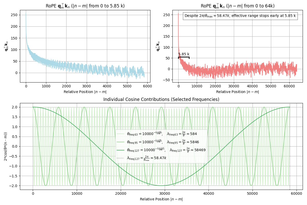
For example, $\lambda_{127}=\frac{2\pi}{\theta_{127}}\approx 58.47\text{k}$
- The HALF wavelength of the highest dimension (the lowest frequency) $\frac{1}{2}\lambda_{\text{longest}}=\frac{\pi}{\theta_{\text{smallest}}}$
By the embedding design philosophy aiming to scale down long distance token attention score, since the half wavelength, the dominant cosine term sees monotonic increase in $[\pi, 2\pi)$ contradicting to this design.
For example, $\frac{1}{2}\lambda_{127}=\frac{\pi}{\theta_{127}}\approx 29.24\text{k}$
Effective RoPE Token Distance Range
See in $\langle \bold{q}_m, \bold{k}_n \rangle$ as token distance $|n-m|$ grows from closely adjacent to faraway,
\[\langle \bold{q}_m, \bold{k}_n \rangle=\sum_{i=0}^{127} \big(\alpha_{\cos}\cos(|n-m|\theta_i)+\alpha_{\sin}\sin(|n-m|\theta_i) \big)\]when tokens are positioned closely the inner product $\langle \bold{q}_m, \bold{k}_n \rangle$ is dominated by cosine $\cos(|n-m|\theta_i)\approx 1$, while sine is trivial $\sin(|n-m|\theta_i)\approx 0$.
As a result, in the beginning the inner product $\langle \bold{q}_m, \bold{k}_n \rangle$ sees monotonic decrease.
As token distance $|n-m|$ grows to longer, e.g., to the $10\%$ of full wavelength $\frac{1}{10}\lambda_{\text{longest}}$, most of dimensions see multiple periods of oscillations over full wavelengths.
For example, out of $D=128$ dimensions, $75\%$ of dimensions have gone through full wavelengths given $\lambda_{95}=\frac{1}{10}\lambda_{127}\approx 5.84\text{k}$.
Together more and more frequencies cancel out each other as token distance $|n-m|$ grows and this results in oscillation convergence around $0$, and since the start of non-decrease oscillation happens, the attention score by $\bold{q}_m^{\top}\bold{k}_n$ no longer holds discriminative semantics.
Proof of Unique Rotary Mapping within $\lambda_d=\frac{2\pi}{\theta_i}$
Assume there are two different angle $\theta_{a}$ and $\theta_{b}$ map to the same rotation $R(\theta_{a})=R(\theta_{b})$. The rotated vector is $\bold{v}\ne\bold{0}\in\mathbb{R}^{2}$.
\[\begin{align*} && \begin{bmatrix} \cos \theta_a & -\sin \theta_a \\ \sin \theta_a & \cos \theta_a \\ \end{bmatrix} \begin{bmatrix} v_x \\ v_y \end{bmatrix} &= \begin{bmatrix} \cos \theta_b & -\sin \theta_b \\ \sin \theta_b & \cos \theta_b \\ \end{bmatrix} \begin{bmatrix} v_x \\ v_y \end{bmatrix} \\ \Rightarrow && \begin{bmatrix} v_x \cos \theta_a - v_y \sin \theta_a \\ v_x \sin \theta_a + v_y \cos \theta_a \\ \end{bmatrix} &= \begin{bmatrix} v_x \cos \theta_b - v_y \sin \theta_b \\ v_x \sin \theta_b + v_y \cos \theta_b \\ \end{bmatrix} \end{align*}\]Consider that $R(\theta)$ is an orthonormal matrix $R^{\top}(\theta)R(\theta)=I$, and inverse property of rotation $R^{-1}(\theta)=R(-\theta)$. Multiply both side by $R^{-1}(\theta)$, there is
\[R(-\theta_a)R(\theta_a)\bold{v}=R(-\theta_a)R(\theta_b)\bold{v}\]Recall the rotation property that counter-clockwise + clockwise same angle rotation is equivalent to no rotation, i.e., $R(-\theta_a)R(\theta_a)=R(\theta_a-\theta_a)=R(0)=I$, hence
\[\bold{v}=R(-\theta_a)R(\theta_b)\bold{v}=\underbrace{R(-\theta_a+\theta_b)}_{=R(0)=I}\bold{v}\]For $\bold{v}=R(-\theta_a+\theta_b)\bold{v}$ to hold, there should be $R(-\theta_a+\theta_b)=R(0)=I$ hence $\theta_a=\theta_b$.
Now reconsider the original hypothesis if it can be assumed that two different angles $\theta_{a}$ and $\theta_{b}$ can map to the same rotation $R(\theta_a)=R(\theta_b)$ on the same $\bold{v}$. The derived expression $\bold{v}=R(-\theta_a+\theta_b)\bold{v}$ led result $\theta_a=\theta_b\in[0, 2\pi)$ rejected the hypothesis.
However, for $R(\theta)=R(\theta+2k\pi), k\in\mathbb{Z}^{+}$ is a periodic function, there can be $\theta_a=\theta_b+2k\pi$, so that two different angles $\theta_{a}$ and $\theta_{b}$ can map to the same rotation. This leads to loss of resolution that resonated two embedding $\bold{v}_m^{\top}\bold{v}_n$ can see multiple mappings. To maintain unique mappings, the highest dimension’s wavelength is essentially the context length.
Appendix: The RoPE Frequency Plot Python Code
import numpy as np
import matplotlib.pyplot as plt
import matplotlib as mpl

# Configuration: 256-dimensional vector gives 128 pairs.
d = 256
pairs = d // 2  # 128 pairs
base = 10000.0

# Compute rotary frequencies for each pair:
# θ_i = 1 / (base^(2*i/d))
freqs = 1.0 / (base ** (2 * np.arange(pairs) / d))

# For the bottom plot, select three frequency indices.
selected_indices = [63, 95, 127]
# x-axis range from 0 to max_wavelength (for the selected lowest frequency)
max_wavelength = (2 * np.pi) / (1/10000**(127/128))
max_wavelength_half = max_wavelength / 2
max_wavelength_tenth = max_wavelength / 10
ps_bottom = np.linspace(0, max_wavelength, num=1000)

# Define relative positions for the upper plots:
# Upper Left: 0 to max_wavelength_tenth
ps1 = np.linspace(0, max_wavelength_tenth, num=2000)
# Upper Right: 0 to 64k
ps2 = np.linspace(0, 64e3, num=2000)

# Compute total dot product for each relative position:
# Each pair contributes 2*cos(θ*(n-m))
dot_total1 = np.array([2 * np.sum(np.cos(p * freqs)) for p in ps1])
dot_total2 = np.array([2 * np.sum(np.cos(p * freqs)) for p in ps2])

# Prepare green colors using the recommended colormap access:
cmap = mpl.colormaps["Greens"]
# We'll choose values between 0.2 (lighter) and 0.6 (darker) for our curves.
norm_values = np.linspace(0.2, 0.6, len(selected_indices))
colors_bottom = [cmap(norm) for norm in norm_values]

# Create the figure with three subplots:
fig = plt.figure(figsize=(12, 8))
# GridSpec: top row has two columns; bottom row spans both.
gs = fig.add_gridspec(2, 2, height_ratios=[1, 1.2])

# Upper Left: Dot Product from 0 to 4k (light blue)
ax1 = fig.add_subplot(gs[0, 0])
ax1.plot(ps1, dot_total1, color="lightblue")
ax1.set_title(r"RoPE $\mathbf{q}^{\top}_m\mathbf{k}_n$ ($|n - m|$ from 0 to %.2f k)" % (max_wavelength_tenth / 1000))
ax1.set_xlabel(r"Relative Position $|n - m|$")
ax1.set_ylabel(r"$\mathbf{q}^{\top}_m\mathbf{k}_n$")
ax1.grid(True)

# Upper Right: Dot Product from 0 to 128k (light coral)
ax2 = fig.add_subplot(gs[0, 1])
ax2.plot(ps2, dot_total2, color="lightcoral")
ax2.set_title(r"RoPE $\mathbf{q}^{\top}_m\mathbf{k}_n$ ($|n - m|$ from 0 to 64k)")
ax2.set_xlabel(r"Relative Position $|n - m|$")
ax2.set_ylabel(r"$\mathbf{q}^{\top}_m\mathbf{k}_n$")
ax2.grid(True)

# --- Add horizontal bracket in the upper right plot ---
# We'll draw the bracket in data coordinates so it sits within the first max_wavelength_tenth region.
# First, get the current y-limits to position the bracket near the top.
y_min, y_max = ax2.get_ylim()
# Place the bracket at 35% of the way from y_min to y_max.
y_bracket = y_min + 0.35*(y_max - y_min)

x_start = 0
x_end = max_wavelength_tenth  # The max_wavelength_tenth region

# Draw a horizontal line for the bracket.
ax2.plot([x_start, x_end], [y_bracket, y_bracket], color='black', lw=2)
# Draw vertical ticks at the ends.
ax2.plot([x_start, x_start], [y_bracket, y_bracket - (y_max-y_min)*0.02], color='black', lw=2)
ax2.plot([x_end, x_end], [y_bracket, y_bracket - (y_max-y_min)*0.02], color='black', lw=2)
# Place the label "max_wavelength_tenth" centered above the bracket.
ax2.text((x_start + x_end) / 2, y_bracket + (y_max-y_min)*0.01, r"%.2f k" % (max_wavelength_tenth / 1000),
         ha="center", va="bottom", fontsize=10)
# --- Add description text to the right of the upper right plot ---
ax2.text(0.95, 0.95, r"Despite $2\pi/\theta_{\text{max}}\approx %.2f k$, effective range stops early at %.2f k" % (max_wavelength / 1000, max_wavelength_tenth / 1000), transform=ax2.transAxes, ha='right', va='top', fontsize=10, bbox=dict(facecolor='white', alpha=0.5))

# Bottom: Individual cosine contributions over 0 to max_wavelength.
ax3 = fig.add_subplot(gs[1, :])
for i, idx in enumerate(selected_indices):
    theta = freqs[idx]
    period = 2 * np.pi / theta  # period for the current frequency
    curve = 2 * np.cos(ps_bottom * theta)
    label = (r"$\theta_{\mathrm{freq}\, %d}=10000^{-\frac{2\, \times %d}{ %d}},\quad "
             r"\lambda_{\mathrm{freq}\, %d}=\frac{2\pi}{\theta}\approx %5d$"
             % (idx, idx, d, idx, period))
    ax3.plot(ps_bottom, curve, label=label, color=colors_bottom[i])

# Draw a vertical dashed line at x = max_wavelength.
dim_max_freq = d/2-1
ax3.axvline(max_wavelength, color='gray', linestyle=':',
    label=r"$\lambda_{\mathrm{freq}\, %d}=\frac{2\pi}{\theta_{\text{max}}}\approx %.2f k$" % (dim_max_freq, max_wavelength / 1000))
ax3.set_title("Individual Cosine Contributions (Selected Frequencies)")
ax3.set_xlabel(r"Relative Position $|n - m|$")
ax3.set_ylabel("2*cos(θ*(n - m))")
ax3.legend()
ax3.grid(True)

plt.tight_layout()
plt.show()