Gaussian Process

April 19, 2025

A Gaussian process is a stochastic process that has a multivariate normal distribution for any finite set of variables.

Reference:

• http://gaussianprocess.org/gpml/chapters/RW.pdf
• https://zhuanlan.zhihu.com/p/75589452

Gaussian Process Derivation

Start from one-dimensional case, there is

\[p(x)=\frac{1}{\sqrt{2\pi\sigma^2}}e^{-\frac{(x-\mu)^2}{2\sigma^2}}\]

where $\mu$ is the mean and $\sigma^2$ is the variance.

For multivariate case, and assume the dimensions are independent, there is

\[\begin{align*} p(\bold{x}) &=p(x_1, x_2, ..., x_n)=\prod_{i=1}^n p(x_i) = \\ &= \frac{1}{\sqrt{(2\pi)^n\sigma^2_1\sigma^2_2...\sigma^2_n}}\exp\bigg(-\frac{1}{2}\Big(\big(\frac{x_1-\mu_1}{\sigma_1}\big)^2+\big(\frac{x_2-\mu_2}{\sigma_2}\big)^2+...+\big(\frac{x_n-\mu_n}{\sigma_n}\big)^2\Big)\bigg) \\ &= \frac{1}{\sqrt{(2\pi)^n\prod_{i=1}^n\sigma^2_i}}\exp\bigg(-\frac{1}{2}\sum_{i=1}^n\big(\frac{x_i-\mu_i}{\sigma_i}\big)^2\bigg) \end{align*}\]

where, similar to one-dimensional case, $\mu_i$ is the mean and $\sigma^2_i$ is the variance with respect to the $i$-th dimension.

let $\bold{x}-\bold{\mu}=[x_1-\mu_1, x_2-\mu_2, …, x_n-\mu_n]^{\top}$, and define the covariance matrix as

\[\Sigma = \begin{bmatrix} \sigma_1^2 & 0 & & 0 \\ 0 & \sigma_2^2 & & 0 \\ & & \ddots & \\ 0 & 0 & & \sigma_n^2 \end{bmatrix}\]

There are

\[\sigma_1\sigma_2...\sigma_n = \sqrt{\det(\Sigma)}=|\Sigma|^{1/2}\]

and,

\[\big(\frac{x_1-\mu_1}{\sigma_1}\big)^2+\big(\frac{x_2-\mu_2}{\sigma_2}\big)^2+...+\big(\frac{x_n-\mu_n}{\sigma_n}\big)^2 = (\bold{x}-\bold{\mu})^{\top}\Sigma^{-1}(\bold{x}-\bold{\mu})\]

so,

\[p(\bold{x}) = \frac{1}{\sqrt{(2\pi)^n|\Sigma|}}\exp\bigg({-\frac{1}{2}(\bold{x}-\bold{\mu})^{\top}\Sigma^{-1}(\bold{x}-\bold{\mu})}\bigg)\]

The above expression can be noted as $\bold{x}\sim\mathcal{N}(\bold{\mu}, \Sigma)$.

Gaussian Process Definition

Define sampling $f(\bold{x})$, that one sample is measured in $n$ dimensions $\bold{x}_i=\left[x_{i1}, x_{i2}, …, x_{in}\right]^{\top}$, and this once sampling result is $f(\bold{x}_i)=[f(x_{i1}), f(x_{i2}), …, f(x_{in})]^{\top}$. There are multiple $n$-dimensional samples $\bold{x}_1, \bold{x}_2, …, \bold{x}_m$, and the sequence of sampling results are $f(\bold{x}_1), f(\bold{x}_2), …, f(\bold{x}_m)$.

This process $f(\bold{x}_1), f(\bold{x}_2), …, f(\bold{x}_m)$ is termed Gaussian process.

RBF Kernel Function

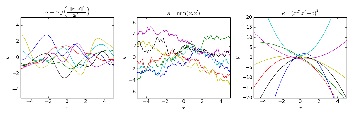
Kernel function determines how Gaussian process is defined, and it RBF (Radial Basis Function) kernel function is a popular kernel function used a covariance matrix to measure the similarity between two samples., and it is defined as

\[\kappa(\bold{x}_i, \bold{x}_j) = \sigma^2\exp\big(-\frac{1}{2l^2}||\bold{x}-\bold{x}'||^2\big)\]

where $l$ is the distance between two samples, and $\sigma^2$ is the variance.

Below are some examples of different kernel functions.

</br>

Gaussian Process Example and Visualization

Assume prior $f(\bold{x})\sim\mathcal{N}(\bold{\mu}_f, \Sigma_{ff})$ follows the Gaussian process, and there are some observation $(\bold{x}^*, \bold{y}^*)$ that are considered following the Gaussian process as well, i.e.,

\[\begin{bmatrix} f(\bold{x}) \\ \bold{y}^* \end{bmatrix} \sim\mathcal{N}\bigg(\begin{bmatrix} \bold{\mu}_f \\ \bold{\mu}_y \end{bmatrix}, \begin{bmatrix} \Sigma_{ff} & \Sigma_{fy} \\ \Sigma_{fy} & \Sigma_{yy} \end{bmatrix}\bigg)\]

As sample size grows, the posterior distribution of the Gaussian process can be calculated by

\[f\sim\mathcal{N}(\Sigma^{\top}_{fy}\Sigma_{ff}^{-1}\bold{y}+\bold{\mu}_f, \Sigma_{ff}-\Sigma^{\top}_{fy}\Sigma_{y}^{-1}\Sigma_{fy})\]

where $\Sigma_{ff}=\kappa(\bold{x}, \bold{x})$, $\Sigma_{fy}=\kappa(\bold{x}, \bold{x}^*)$, $\Sigma_{yy}=\kappa(\bold{x}^*, \bold{x}^*)$. Here uses RBF as kernel function $\kappa(\bold{x}, \bold{x}’)$.

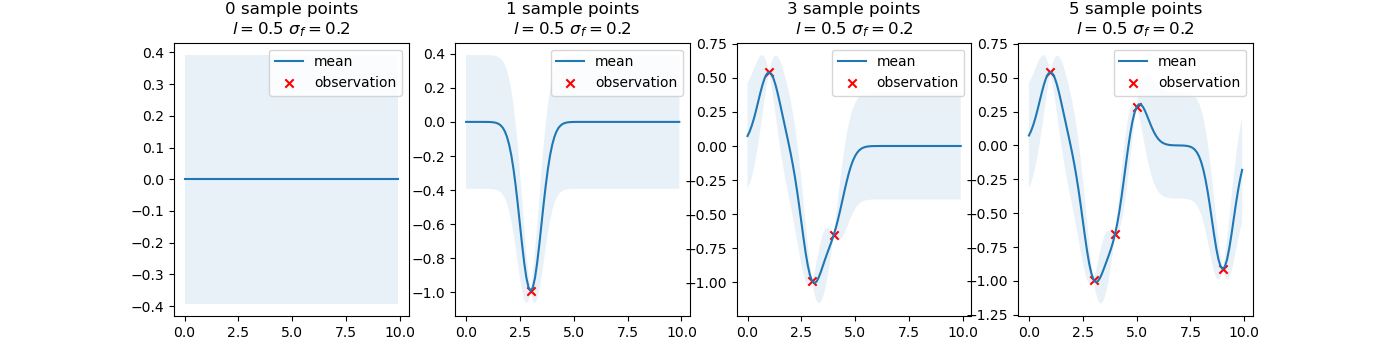
In the figure below, the Gaussian process starts from the prior distribution with $\mu_f=\bold{0}$ and $\Sigma_{ff}=\sigma_f^2I$. Then, when the first sampling is done, the neighboring samples are considered to be close to the first sampling point. As more and more observations are added, in the neighbor area of observation points, the Gaussian process shows high-level certainty, while in the sparse areas, the Gaussian process shows low-level certainty.

The uncertainty is measured by the shaded area, which is the variance ($95\%$ confidence interval) of the Gaussian process.

</br>

Here plots five possible $f(.)$s that follow the Gaussian process passing through the observation points.

\[f\sim\mathcal{N}(\Sigma^{\top}_{fy}\Sigma_{ff}^{-1}\bold{y}+\bold{\mu}_f, \Sigma_{ff}-\Sigma^{\top}_{fy}\Sigma_{y}^{-1}\Sigma_{fy})\]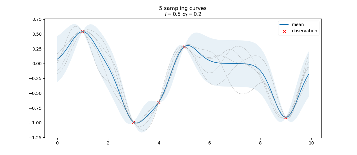

</br>

Gaussian Process Optimization

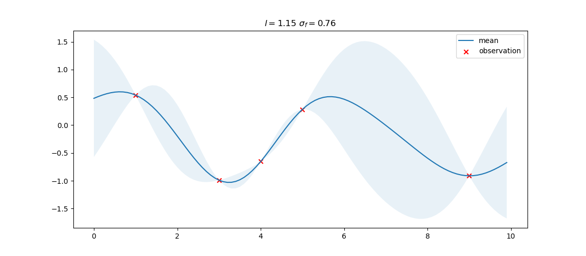
In the above example, the Gaussian process is defined with static $l=0.5$ and $\sigma_f=0.2$, however, in practice, they can be optimized by maximizing the likelihood.

\[\begin{align*} \min\log p(\bold{y}|\bold{x}) &= \log\mathcal{N}\big(\bold{0}, \Sigma_{yy}(\sigma, l)\big) \\ &= \frac{1}{2}\log|\Sigma_{yy}(\sigma, l)|+\frac{1}{2}\bold{y}^{\top}\Sigma_{yy}(\sigma, l)^{-1}\bold{y} \end{align*}\]

where $\Sigma_{yy}=\kappa(\bold{x}^*, \bold{x}^*)$.

The optimization result is shown below, where $l=1.15$ and $\sigma_f=0.76$. The optimization result has a smoothing effect as exemplified in the shaded area.

</br>