Linear Transform Intuition

March 14, 2025

Example Calculations and Intuition

Linear Transform Intuition Given Eigenvectors and Eigenvalues

To find eigenvalues and eigenvectors for $A$ as given

Solution:

hence $\lambda_1 = 1$ and $\lambda_2 = 3$.

for eigenvectors:

thus derived

same calculation applied when $\lambda = 3$

Geometrically speaking, the transformation matrix $A$ can be explained as scaling with a multiple of \(1\) on \(\bold{v}_{\lambda_1}\) and \(3\) on \(\bold{v}_{\lambda_2}\) basis.

For example, there exist points by transform $A\bold{x}_i$:

• $\bold{x}_1=(1,3)$, there is $A\bold{x}_1=(7,5)$
• $\bold{x}_2=(1,2)$, there is $A\bold{x}_2=(5,4)$
• $\bold{x}_3=(1,1)$, there is $A\bold{x}_3=(3,3)$, exactly scaled by $\lambda_2=3$
• $\bold{x}_4=(1,0)$, there is $A\bold{x}_4=(2,1)$
• $\bold{x}_5=(1,-1)$, there is $A\bold{x}_5=(1,-1)$, exactly scaled by $\lambda_1=1$
• $\bold{x}_6=(1,-2)$, there is $A\bold{x}_6=(0,-3)$
• $\bold{x}_7=(1,-3)$, there is $A\bold{x}_7=(-1,-5)$

</br>

In conclusion, the larger value of eigenvalue, the more powerful it could stretch linear transform towards the corresponding eigenvector direction. If a point sits exactly on an eigenvector, this point is stretched linearly by eigenvalue on the eigenvector direction.

import numpy as np
import matplotlib.pyplot as plt
import matplotlib.animation as animation

# Define the transformation matrix A
A = np.array([[2, 1], [1, 2]])

# Define the original points
points = np.array([
    [1, 3],
    [1, 2],
    [1, 1],
    [1, 0],
    [1, -1],
    [1, -2],
    [1, -3]
])

# Compute transformed points
transformed_points = np.dot(points, A.T)

# Eigenvectors and eigenvalues
eigenvalues, eigenvectors = np.linalg.eig(A)

# Animation setup
fig, ax = plt.subplots()
ax.set_xlim(-2, 12)
ax.set_ylim(-6, 6)
ax.set_xlabel("x")
ax.set_ylabel("y")
ax.grid()

# Plot x and y axes
ax.axhline(0, color='black', linewidth=1)
ax.axvline(0, color='black', linewidth=1)

# Plot eigenvectors
for i in range(2):
    vec = eigenvectors[:, i] * eigenvalues[i]  # Scale for better visualization
    ax.plot([-vec[0], vec[0]], [-vec[1], vec[1]], color='plum', linestyle='dashed',
            label=f"Eigenvector [%.3f %.3f], Eigenvalue %.3f" %
                    (eigenvectors[0, i], eigenvectors[1, i], eigenvalues[i]))
# Plot original points
scatter_original, = ax.plot(points[:, 0], points[:, 1], 'o', color='lightblue', label="Original Points")
scatter_transformed, = ax.plot([], [], 'o', color='lightgreen', label="Transforming Points")
ax.legend(loc='lower right')

# Animate transformation
def update(frame):
    t = frame / 30  # interpolation factor (0 to 1)
    intermediate_points = (1 - t) * points + t * transformed_points
    scatter_transformed.set_data(intermediate_points[:, 0], intermediate_points[:, 1])
    return scatter_transformed,

ani = animation.FuncAnimation(fig, update, frames=31, interval=50, blit=True)

# Save the animation as a GIF
ani.save("linear_transform_example.gif", writer="pillow", fps=15)

plt.show()

Calculate Matrix With Stacked Powered Matrix

Solution:

Calculate inverse:

Use $e$ log:

get the eigenvalues and eigenvectors

for

thus,

thus

Consider the original equation

then

again, get the eigenvalues and eigenvectors

for

thus

thus, derived the final solution

Covariance Matrix

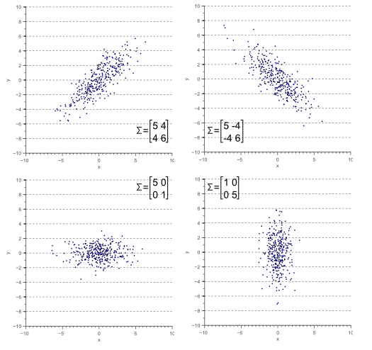
A $2 \times 2$ covariance matrix is defined as

in which \(\sigma(x,y) = E [ \big(x - E(x) \big) \big(y - E(y)\big) ]\)

where $x$ and $y$ are sample vectors, hence $\sigma(x,y)$ is scalar.

</br>

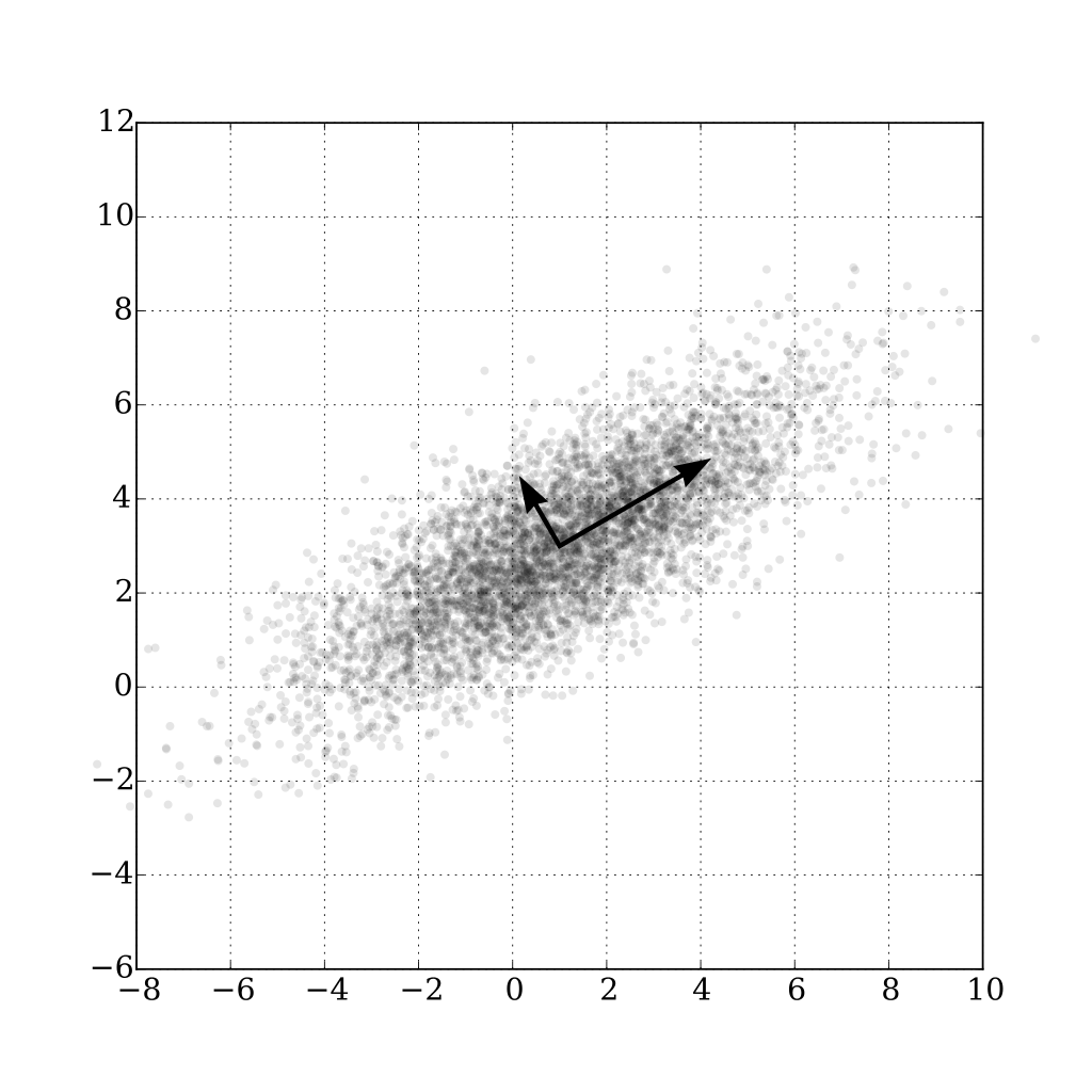
The orientations and thickness of the point cloud are eigenvectors and eigenvalues, such as the two arrows shown as below.

</br>

Determinant And Trace (Indicative of Transform Volume)

Determinant

The determinant of a square matrix $A$ representing a linear transformation is a scalar value that quantifies the factor by which the transformation scales volumes in space.

$\text{det}(A)>1$ Expansion

$\text{det}(A)<1$ Contraction

$\text{det}(A)=1$ Volume Preservation/Pure Rotation

The vector $\bold{x}$ is rotated by $90$ degrees counterclockwise.

$\text{det}(A)=0$ Collapse

$\text{det}(A)=0$ happens when $\text{rank}(A)$ is not full.

All $\bold{x}_i$ are collapsed into the line $0=x_2-x_1$.

Trace

Trace of a matrix is defined as

A matrix trace equals the dum of its diagonal entries and the sum of Its eigenvalues.

Since matrix trace is the sum of eigenvalues, it shows a vague overview of eigenvalue “energy”.

Determinant shows more detailed how matrix transformation volume expands/contracts, however, is much more difficult to compute. Trace comes in rescue as an alternative characterized by easy computation.

Infinitesimal Transformations and Linear Approximation

For $A$ close to the identity (i.e., $I+\epsilon A$, where $\epsilon$ is a trivial amount), the first-order approximation of the determinant is $\text{det}(I+\epsilon A)=1+\epsilon \text{tr}(A)$. For $\epsilon$ is a trivial amount, higher-order terms can be dropped/ignored.

Thus, $\text{tr}(A)$ approximates the volume change rate for small $\epsilon$.

Example: Rate of Continuous Dynamical Linear Systems

Consider a linear continuous dynamical system defined by $\frac{d\bold{x}}{dt}=A\bold{x}$, its integration solution is $\bold{x}(t)=e^{At}\bold{x}(0)$.

The volume scaling factor over time $t$ is $\text{det}(e^{At})=e^{\text{tr}(A)t}$. Differentiating at $t=0$, the instantaneous rate of volume change is $\frac{d}{dt}\text{det}(e^{At})\big|_{t=0}=\text{tr}(A)$.

Take iterative steps to update the dynamic linear system by $t_{+1}=t_{0}+\delta t$, and remember $\frac{d\bold{x}}{dt}=A\bold{x}$ is real time computation given at the time input $\bold{x}$ (the observed change $A\bold{x}$ is different per each timestamp observation at $t_0$). When $\delta t\rightarrow 0$ is small enough, the dynamic system can be viewed continuous at every $t_{0}\rightarrow t_{+1}$ with the change rate $\text{tr}(A)$.

In conclusion, $\text{tr}(A)$ is the first-order/linear approximation over time at every system update step $t_{+1}=t_{0}+\delta t$.

Volume Growth/Decay:

• If $\text{tr}⁡(A)>0$: Volume expands exponentially.
• If $\text{tr}⁡(A)<0$: Volume contracts exponentially.
• If $\text{tr}⁡(A)=0$: Volume is preserved (e.g., Hamiltonian systems).

Eigenvector and Orthogonality

If $A^{\top}A=I$, matrix $A$ is termed orthogonal matrix.

An orthogonal matrix preserves vector length and inner product (the result is invariant) during linear transformation.

For example, a rotation matrix is orthogonal.

Eigen-Decomposition (Diagonalization)

Eigen-decomposition (diagonalization) breaks a square matrix $A$ into eigenvectors and eigenvalues.

where

• $\Lambda$: a diagonal matrix where non-zero entries are eigenvalues
• $Q$: Matrix whose columns are eigenvectors of $A$

It has the properties: $Q^{\top}=Q$, so that $Q^{-1}=Q$.

For a matrix eigen-decomposition that the resultant eigenvectors are orthogonal, there are a few scenarios and conditions.

Real Symmetry and Eigenvector Orthogonality

A matrix is real symmetric if $A^{\top}=A\in\mathbb{R}^{n \times n}$.

By the Spectral Theorem, if $A$ is a real symmetric matrix, then:

• All eigenvalues of $A$ are real
• This means the eigenvectors of $A$ can be chosen to be orthogonal and normalized.
• $A$ can be can be orthogonally diagonalized $A=Q\Lambda Q^{\top}$, where 1) $\Lambda$ is a diagonal matrix containing the eigenvalues of $A$, 2) the columns of $Q$ are the orthonormal eigenvectors of $A$.