Singular Value Decomposition (SVD)
April 14, 2025
SVD is a factorization that decompose an $m \times n$ matrix A into
\[A=U \Sigma V^{\top}\]SVD generalizes the eigen-decomposition of a square normal matrix with an orthonormal eigen basis to any $n \times m$ matrix $A$.
SVD Derivation
Compute the eigenvalues and eigenvectors of $A^{\top}A$
\[A^{\top}A \bold{v}_1 = \sigma_1^2 \bold{v}_1 \\ A^{\top}A \bold{v}_2 = \sigma_2^2 \bold{v}_2 \\ ... \\ A^{\top}A \bold{v}_n = \sigma_n^2 \bold{v}_n\]- So that $V$ is
- So that $\Sigma$ is
or (depending on the relative matrix sizes of $m$ vs $n$)
\[\Sigma= \begin{bmatrix} \sigma_1 & & \\ & \ddots & \\ & & \sigma_n \\ & \bold{0} & \end{bmatrix}\]- So that $U$ is
Proof of Orthogonality
$A^{\top}A$ is Symmetric Hence $V$ Is Orthogonal
Define follows for $i\ne j$
\[A^{\top}A\bold{v}_i=\sigma_i^2\bold{v}_i \qquad A^{\top}A\bold{v}_j=\sigma_j^2\bold{v}_j\]then multiply by $\bold{v}_j^{\top}$, there is
\[\begin{align*} && \bold{v}_j^{\top}A^{\top}A\bold{v}_i &= \bold{v}_j^{\top}\sigma_i^2\bold{v}_i \\ \Rightarrow && (A^{\top}A\bold{v}_j)^{\top}\bold{v}_i &= \bold{v}_j^{\top}\sigma_i^2\bold{v}_i \qquad\text{ for symmetry } \big(A^{\top}A\big)^{\top}=A^{\top}A \\ \Rightarrow && \sigma_j^2\bold{v}_j^{\top}\bold{v}_i &= \sigma_i^2\bold{v}_j^{\top}\bold{v}_i \\ \end{align*}\]For by eigen-decomposition, there is $\sigma_i^2 \ne \sigma_j^2 \ne 0$, there could be only $\bold{v}_j^{\top}\bold{v}_i=0$, hence orthogonal.
For ${\bold{v}_1, \bold{v}_2, …, \bold{v}_n}$ are defined as eigenvectors of $A$ such that $V=\begin{bmatrix} \vdots & & \vdots \ \bold{v}_1 & … & \bold{v}_n \ \vdots & & \vdots \end{bmatrix}$, $V$ is orthogonal.
$U$ Is Orthogonal For It Is Equivalent of $V$ For $AA^{\top}$
For $A^{\top}A=Q\Sigma Q^{\top}$ established by spectral theorem that for symmetric matrix eigen-decomposition, $Q$ is orthogonal. The difference is that the spectral theorem only works for square matrix, while SVD works for non-square matrix as well.
The non-square matrix $A\in\mathbb{R}^{n\times m}$ has diff sizes for $A^{\top}A\in\mathbb{R}^{m\times m}$ vs $AA^{\top}\in\mathbb{R}^{n\times n}$, as a result, for $A^{\top}A=V\Sigma V^{\top}$, there is equivalent $AA^{\top}=U\Sigma U^{\top}$.
In conclusion, $U$ is orthogonal for it is equivalent of $V$ for $AA^{\top}$ and is of different size.
Intuition of SVD by Geometry
In geometry intuition in $A=U \Sigma V^{\top}$, the $U$ and $V^{\top}$ are considered reflection/rotation, and $\Sigma$ is a scaling matrix.
$V$ and $U$ As Reflection/Rotation
- If $\text{det}(V)=-1$, it is a reflection.
- If $\text{det}(V)=1$, it is a rotation.
This is for that
1) For $|\text{det}(V)|=1$, there is no scaling. 2) For $\text{det}(V)>0$, orientation is preserved. 3) For $\text{det}(V)<0$, orientation is reversed.
- During reflection/rotation, the linear space angle is preserved.
Given two input vectors $\bold{x}_i$ and $\bold{x}_j$, the angle between them satisfies $\cos(\theta)=\frac{\bold{x}_i^{\top}\bold{x}_j}{||\bold{x}_i||\space||\bold{x}_i||}$. Apply the orthonormal matrix $V$, there is
\[\cos(\theta')=\frac{(V\bold{x}_i)^{\top}V\bold{x}_j}{||V\bold{x}_i||\space||V\bold{x}_i||}= \frac{\bold{x}_i^{\top}\bold{x}_j}{||\bold{x}_i||\space||\bold{x}_i||}= \cos(\theta)\]Thus, $\theta’=\theta$, the angle is preserved.
This holds true for $U$ as well.
$\Sigma$ As Scaling
$\Sigma$ is a diagonal matrix, hence its non-zero entries act as pure scaling.
SVD Explanation by Geometry
Let $\bold{x}_i=[3, 3]$ and $\bold{x}_i=[3, 1]$ that are transformed by $A=\begin{bmatrix} -1 & 1 \ 0 & 1 \end{bmatrix}$. Below process shows how $A\bold{x}=U \Sigma V^{\top}\bold{x}$ is computed.
- For $\text{det}(V)=-1$, the $V^{\top}\bold{x}$ is a reflection operation.
- For $\Sigma$ is a diagonal matrix, the $\Sigma V^{\top}\bold{x}$ is a scaling operation.
- For $\text{det}(U)=1$, the $U\Sigma V^{\top}\bold{x}$ is a rotation operation.
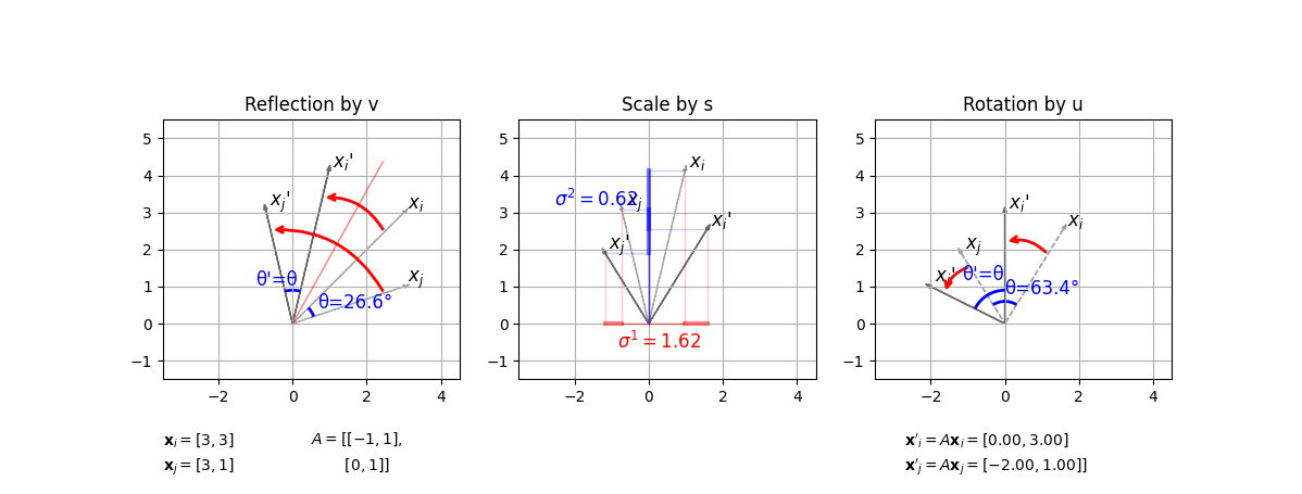
</br>
where during reflection and rotation, the angle $\theta’=\theta$ is preserved.
SVD in Machine Learning
Typically, for a population of samples $A$, the covariance ${\Omega}$ of $A$ (typically use ${\Sigma}$ as covariance matrix notation, but here use ${\Omega}$ to avoid duplicate notations as ${\Sigma}$ means singular value matrix in this article) of the samples’ features describes how rich information they are. Larger the variance of a feature, likely richer the information.
Take SVD on the covariance matrix such that ${\Omega}=U \Sigma V^\top$, and obtain singular value matrix ${\Sigma}$ and new orthogonal basis space $V$. Intuitively speaking, ${\Sigma}$ describes how significant is for each corresponding orthogonal basis vector in $V$.
The transformed new orthogonal space $V$ can help recover the source sample data by $A=AV$.
SVD for PCA
PCA (Principal Component Analysis) simply takes the first few most significant components out of the result of SVD (Singular Value Decomposition).
SVD for Least Squares Problem
Given a least squares problem: for a residual $\bold{r} = A \bold{x} - \bold{b}$, where $A \in \mathbb{R}^{m \times n}$ (assumed $A$ is full rank that $n = \text{rank}(A)$), and there is $m > n$, here attempts to minimize
\[\space \underset{\bold{x}}{\text{min}} \space ||A \bold{x} - \bold{b}||^2= r_1^2 + r_2^2 + ... + r^2_m\]Process:
\[\begin{align*} & ||A \bold{x} - \bold{b}||^2 \\ =& ||U \Sigma V^{\top} \bold{x} - \bold{b}||^2 \\ =& ||U^{\top}(U \Sigma V^{\top} \bold{x} - \bold{b})||^2 \\ =& ||U^{\top}U \Sigma V^{\top} \bold{x} - U^{\top}\bold{b}||^2 \quad U\text{ is orthoganal that } U^{\top}U=I\\ =& ||\Sigma V^{\top} \bold{x} - U^{\top}\bold{b}||^2\\ =& ||\Sigma \bold{y} - U^{\top}\bold{b}||^2 \quad \text{denote } \bold{y}=V^\top\bold{x} \text{ and } \bold{z}=U^\top\bold{b} \\ =& \Bigg|\Bigg| \begin{bmatrix} \sigma_1 & & & \\ & \ddots & & \\ & & \sigma_n & \\ & & & \bold{0} \end{bmatrix} \bold{y} - \bold{z} \Bigg|\Bigg|^2\\ =& \sum^{n}\_{i=1} \big( \sigma_i {y}_i - \bold{u}^{\top}_i \bold{b} \big)^2+\sum^{m}\_{i=n+1} \big( \bold{u}^{\top}_i \bold{b} \big)^2 \end{align*}\]$\bold{y}$ is determined as
\[y_i= \left\{ \begin{array}{cc} \frac{\bold{u}^{\top}_i \bold{b}}{\sigma_i} &\quad \sigma_i \ne 0 \text{ same as } i \le n \\ \text{any value} &\quad \sigma_i = 0 \text{ same as } i > n \end{array} \right.\]Then, it is easy to find $\bold{x}$ by $\bold{x} = V\bold{y}$.
The residual is $\sum^{m}_{i=n+1} \big( \bold{u}^{\top}_i \bold{b} \big)^2$.
Proof of SVD as Solution for Least Squares Problem
In the above obtained $||A \bold{x} - \bold{b}||^2=\sum^{n}_{i=1} \big( \sigma_i {y}_i - \bold{u}^{\top}_i \bold{b} \big)^2+\sum^{m}_{i=n+1} \big( \bold{u}^{\top}_i \bold{b} \big)^2$, the second residual term $\sum^{m}_{i=n+1} \big( \bold{u}^{\top}_i \bold{b} \big)^2$ does not depend on $\bold{y}$, so it is simply the irreducible residual.
The first sum reaches its minimum $0=\sum^{n}_{i=1} \big( \sigma_i {y}_i - \bold{u}^{\top}_i \bold{b} \big)^2$ with $y_i=\frac{\bold{u}^{\top}_i \bold{b}}{\sigma_i}$.
SVD vs Eigen Decomposition
-
SVD generalizes the eigen decomposition of a square normal matrix with an orthonormal eigen basis to any $m \times n$ matrix.
-
Eigen decomposition: not necessarily orthonormal vs SVD: orthonormal
Here defines a typical linear system $A\bold{x}=\bold{b}$. Consider the eigen decomposition $A = P\Lambda P^{-1}$ and $A=U\Sigma V^{\top}$.
Eigen decomposition only takes one basis $P$ in contrast to SVD using two bases $U$ and $V$. Besides, $P$ might not be orthogonal but $U$ and $V$ are orthonormal (orthogonal + unitary).
Real Symmetry and Eigenvector Orthogonality
A matrix is real symmetric if $A^{\top}=A\in\mathbb{R}^{n \times n}$.
By the Spectral Theorem, if $A$ is a real symmetric matrix, then:
- All eigenvalues of $A$ are real
- This means the eigenvectors of $A$ can be chosen to be orthogonal and normalized.
- $A$ can be can be orthogonally diagonalized $A=P\Lambda P^{\top}$, where 1) $\Lambda$ is a diagonal matrix containing the eigenvalues of $A$, 2) the columns of $P$ are the orthonormal eigenvectors of $A$.
Code for SVD Explanation by Geometry
import numpy as np
import matplotlib.pyplot as plt
from matplotlib.patches import Arc

# 1) Define two vectors
x_i = np.array([3, 3])
x_j = np.array([3, 1])

# 2) Define matrix A, compute its SVD, get V, and build rotation matrix R
A = np.array([[-1, 1], [0, 1]])
U, S, Vt = np.linalg.svd(A)
S = np.diag(S)

# 2.2) Compute for reflection/rotation for V and U
def compute_vec_change_ang(mat):
    mat_det = np.linalg.det(mat)
    print(f"det({mat})={mat_det}")
    if mat_det == 1.0:
        change_ang = np.arctan2(mat[1, 0], mat[0, 0])
    else:
        eigvals, eigvecs = np.linalg.eig(mat)
        axis_idx = np.where(np.isclose(eigvals, 1))[0][0]
        n = eigvecs[:, axis_idx]
        n = n / np.linalg.norm(n)  # Ensure unit vector
        I = np.eye(2)
        change_ang = I - 2 * np.outer(n, n)
    return change_ang
change_ang_v = compute_vec_change_ang(Vt)
change_ang_u = compute_vec_change_ang(U)

# 3) Transform by SVD
x_i_v = Vt @ x_i
x_j_v = Vt @ x_j
x_i_s = S @ Vt @ x_i
x_j_s = S @ Vt @ x_j
x_i_u = U @ S @ Vt @ x_i
x_j_u = U @ S @ Vt @ x_j


# Find max/min to plot
x_min, y_min = -3, -1
x_max, y_max = 4, 5

# Add some padding to the limits
padding = 0.5
x_min -= padding
x_max += padding
y_min -= padding
y_max += padding

# 4) Compute absolute angles for drawing arcs
ang_i = np.degrees(np.arctan2(x_i[1], x_i[0]))
ang_j = np.degrees(np.arctan2(x_j[1], x_j[0]))
ang_i_v = np.degrees(np.arctan2(x_i_v[1], x_i_v[0]))
ang_j_v = np.degrees(np.arctan2(x_j_v[1], x_j_v[0]))
ang_i_s = np.degrees(np.arctan2(x_i_s[1], x_i_s[0]))
ang_j_s = np.degrees(np.arctan2(x_j_s[1], x_j_s[0]))
ang_i_u = np.degrees(np.arctan2(x_i_u[1], x_i_u[0]))
ang_j_u = np.degrees(np.arctan2(x_j_u[1], x_j_u[0]))

# 5) Compute preserved angle θ' (should equal θ)
theta_original = np.arccos(
    np.dot(x_i, x_j) /
    (np.linalg.norm(x_i) * np.linalg.norm(x_j))
)
theta_v = np.arccos(
    np.dot(x_i_v, x_j_v) /
    (np.linalg.norm(x_i_v) * np.linalg.norm(x_j_v))
)
theta_s = np.arccos(
    np.dot(x_i_s, x_j_s) /
    (np.linalg.norm(x_i_s) * np.linalg.norm(x_j_s))
)
theta_u = np.arccos(
    np.dot(x_i_u, x_j_u) /
    (np.linalg.norm(x_i_u) * np.linalg.norm(x_j_u))
)

# 6) Plot
fig, axs = plt.subplots(nrows=1, ncols=3, figsize=(9, 3))

def plot_ax(ax, x_i, x_j, x_i_new, x_j_new,
            ang_i, ang_j, ang_i_new, ang_j_new,
            change_ang,
            flag='v'):

    # Original vectors (dashed gray)
    ax.arrow(0, 0, *x_i, head_width=0.1, linestyle='--', color='gray', alpha=0.7)
    ax.arrow(0, 0, *x_j, head_width=0.1, linestyle='--', color='gray', alpha=0.7)

    # Rotated vectors x' (solid dark gray)
    ax.arrow(0, 0, *x_i_new, head_width=0.1, color='dimgray', alpha=1.0)
    ax.arrow(0, 0, *x_j_new, head_width=0.1, color='dimgray', alpha=1.0)

    # Labels
    ax.text(x_i[0]+0.1, x_i[1]+0.1, '$x_i$', fontsize=12)
    ax.text(x_j[0]+0.1, x_j[1]+0.1, '$x_j$', fontsize=12)
    ax.text(x_i_new[0]+0.1, x_i_new[1]+0.1, "$x_i$'", fontsize=12)
    ax.text(x_j_new[0]+0.1, x_j_new[1]+0.1, "$x_j$'", fontsize=12)

    if flag == 'v' or flag == 'u':
        if flag == 'v':
            ax.set_title(f'Reflection by {flag}')
            theta_p = theta_v
            theta = theta_original
        else:
            ax.set_title(f'Rotation by {flag}')
            theta_p = theta_u
            theta = theta_s

        if ang_i > ang_j:
            ang_i, ang_j = ang_j, ang_i
        if ang_i_new > ang_j_new:
            ang_i_new, ang_j_new = ang_j_new, ang_i_new

        # Arcs for θ and θ' (blue)
        r_theta = 0.6
        arc_theta = Arc((0, 0), 2*r_theta, 2*r_theta,
                        angle=0, theta1=ang_i, theta2=ang_j,
                        color='blue', lw=2)
        ax.add_patch(arc_theta)

        r_theta2 = 0.9
        arc_theta2 = Arc((0, 0), 2*r_theta2, 2*r_theta2,
                        angle=0, theta1=ang_i_new, theta2=ang_j_new,
                        color='blue', lw=2)
        ax.add_patch(arc_theta2)

        if not isinstance(change_ang, np.ndarray):
            change_ang_i = change_ang
            change_ang_j = change_ang
            r_phi = 2.2
            start = (r_phi * np.cos(np.radians(ang_i)),
                    r_phi * np.sin(np.radians(ang_i)))
            end = (r_phi * np.cos(np.radians(ang_i + np.degrees(change_ang_i))),
                r_phi * np.sin(np.radians(ang_i + np.degrees(change_ang_i))))
            ax.annotate(
                '', xy=end, xytext=start,
                arrowprops=dict(arrowstyle='->', lw=2, color='red',
                                connectionstyle="arc3,rad=0.3")
            )
            r_phi = 1.8
            start = (r_phi * np.cos(np.radians(ang_j)),
                    r_phi * np.sin(np.radians(ang_j)))
            end = (r_phi * np.cos(np.radians(ang_j + np.degrees(change_ang_j))),
                r_phi * np.sin(np.radians(ang_j + np.degrees(change_ang_j))))
            ax.annotate(
                '', xy=end, xytext=start,
                arrowprops=dict(arrowstyle='->', lw=2, color='red',
                                connectionstyle="arc3,rad=0.3")
            )
        else:
            # Compute the outer product component
            diff_matrix = (np.eye(2) - change_ang) / 2

            # Extract n from the first non-zero column
            n_column = diff_matrix[:, 0] if np.any(diff_matrix[:, 0]) else diff_matrix[:, 1]
            n = n_column / np.linalg.norm(n_column)
            angle_normal = np.arctan2(n[1], n[0])  # Angle of the normal vector

            # Ensure the angle is within [0, 2π)
            reflection_angle = (2* angle_normal) % (2 * np.pi)

            ax.plot([0, n[0] * (x_max+y_max)/2 ], [0, n[1] * (x_max+y_max)/2 ], color='red',
                    linewidth=1, alpha=0.5, zorder=2)

            r_phi = 2.6
            start = (r_phi * np.cos(np.radians(ang_i)),
                    r_phi * np.sin(np.radians(ang_i)))
            end = (r_phi * np.cos(np.radians(np.degrees(reflection_angle)-ang_i)),
                r_phi * np.sin(np.radians(np.degrees(reflection_angle)-ang_i)))
            ax.annotate(
                '', xy=end, xytext=start,
                arrowprops=dict(arrowstyle='->', lw=2, color='red',
                                connectionstyle="arc3,rad=0.3")
            )
            r_phi = 3.5
            start = (r_phi * np.cos(np.radians(ang_j)),
                    r_phi * np.sin(np.radians(ang_j)))
            end = (r_phi * np.cos(np.radians(np.degrees(reflection_angle)-ang_j)),
                r_phi * np.sin(np.radians(np.degrees(reflection_angle)-ang_j)))
            ax.annotate(
                '', xy=end, xytext=start,
                arrowprops=dict(arrowstyle='->', lw=2, color='red',
                                connectionstyle="arc3,rad=0.3")
            )

        # Labels on arcs
        mid_theta = ang_i + (ang_j - ang_i)/2
        ax.text(r_theta * np.cos(np.radians(mid_theta)) * 1.3,
                r_theta * np.sin(np.radians(mid_theta)) * 1.3,
                f'θ={np.degrees(theta):.1f}°',
                color='blue', fontsize=12)

        mid_theta2 = ang_i_new + np.degrees(theta_p)/2
        ax.text(r_theta2 * np.cos(np.radians(mid_theta2)+1) * 1.3,
                r_theta2 * np.sin(np.radians(mid_theta2)-0.5) * 1.3,
                f"θ'=θ",
                color='blue', fontsize=12)

    elif flag == 's':
        ax.set_title(f'Scale by {flag}')

        # Add bold lines along x and y axes indicating scaling factors
        sigma_x = S[0, 0]
        sigma_y = S[1, 1]

        x_i_0_sig = sigma_x * x_i[0]
        x_i_1_sig = sigma_y * x_i[1]
        x_j_0_sig = sigma_x * x_j[0]
        x_j_1_sig = sigma_y * x_j[1]

        # X-axis line (red)
        ax.plot([x_i[0], x_i_0_sig], [0, 0], color='red', linewidth=3, alpha=0.5, zorder=2)
        ax.plot([x_j[0], x_j_0_sig], [0, 0], color='red', linewidth=3, alpha=0.5, zorder=2)
        ax.plot([0, x_i[0]], [0, 0], color='red', linewidth=1, alpha=0.5, zorder=2)
        ax.plot([0, x_j[0]], [0, 0], color='red', linewidth=1, alpha=0.5, zorder=2)
        # Y-axis line (blue)
        ax.plot([0, 0], [x_i[1], x_i_1_sig], color='blue', linewidth=3, alpha=0.5, zorder=2)
        ax.plot([0, 0], [x_j[1], x_j_1_sig], color='blue', linewidth=3, alpha=0.5, zorder=2)
        ax.plot([0, 0], [0, x_i[1]], color='blue', linewidth=1, alpha=0.5, zorder=2)
        ax.plot([0, 0], [0, x_j[1]], color='blue', linewidth=1, alpha=0.5, zorder=2)
        # Align Y-axis line (blue)
        ax.plot([x_i[0], 0], [x_i[1], x_i[1]], color='blue', linewidth=1, alpha=0.2, zorder=2)
        ax.plot([x_i_new[0], 0], [x_i_new[1], x_i_new[1]], color='blue', linewidth=1, alpha=0.2, zorder=2)
        ax.plot([x_j[0], 0], [x_j[1], x_j[1]], color='blue', linewidth=1, alpha=0.2, zorder=2)
        ax.plot([x_j_new[0], 0], [x_j_new[1], x_j_new[1]], color='blue', linewidth=1, alpha=0.2, zorder=2)
        # Align X-axis line (red)
        ax.plot([x_i[0], x_i[0]], [0, x_i[1]], color='red', linewidth=1, alpha=0.2, zorder=2)
        ax.plot([x_i_new[0], x_i_new[0]], [0, x_i_new[1]], color='red', linewidth=1, alpha=0.2, zorder=2)
        ax.plot([x_j[0], x_j[0]], [0, x_j[1]], color='red', linewidth=1, alpha=0.2, zorder=2)
        ax.plot([x_j_new[0], x_j_new[0]], [0, x_j_new[1]], color='red', linewidth=1, alpha=0.2, zorder=2)

        # Labels for sigma values
        ax.text((x_i[0]+x_i_0_sig)/2-1.0, -0.2, f'$σ^1={sigma_x:.2f}$', color='red', ha='center', va='top', fontsize=12, zorder=4)
        ax.text(-0.3, (x_i[1]+x_i_1_sig)/2, f'$σ^2={sigma_y:.2f}$', color='blue', ha='right', va='center', fontsize=12, zorder=4)

    ax.set_aspect('equal')
    ax.grid(True)

plot_ax(axs[0], x_i, x_j, x_i_v, x_j_v,
        ang_i, ang_j, ang_i_v, ang_j_v,
        change_ang_v,
        flag='v')
plot_ax(axs[1], x_i_v, x_j_v, x_i_s, x_j_s,
        ang_i_v, ang_j_v, ang_i_s, ang_j_s,
        change_ang_v,
        flag='s')
plot_ax(axs[2], x_i_s, x_j_s, x_i_u, x_j_u,
        ang_i_s, ang_j_s, ang_i_u, ang_j_u,
        change_ang_u,
        flag='u')

# Set the same limits for all axes
for ax in [axs[0], axs[1], axs[2]]:
    ax.set_xlim(x_min, x_max)
    ax.set_ylim(y_min, y_max)

axs[0].text(0.0, -0.2,
            f"$\\mathbf_i = [{x_i[0]}, {x_i[1]}]$",
            ha='left', va='top', transform=axs[0].transAxes)
axs[0].text(0.0, -0.3,
            f"$\\mathbf_j = [{x_j[0]}, {x_j[1]}]$",
            ha='left', va='top', transform=axs[0].transAxes)
axs[0].text(0.5, -0.2,
            f"$A=[[{A[0, 0]}, {A[0, 1]}],$",
            ha='left', va='top', transform=axs[0].transAxes)
axs[0].text(0.5, -0.3,
            f"       $[{A[1, 0]}, {A[1, 1]}]]$",
            ha='left', va='top', transform=axs[0].transAxes)

axs[2].text(2.4, -0.2,
            f"$\\mathbf'_i=A\\mathbf_i = [{x_i_u[0]:.2f}, {x_i_u[1]:.2f}]$",
            ha='left', va='top', transform=axs[0].transAxes)
axs[2].text(2.4, -0.3,
            f"$\\mathbf'_j=A\\mathbf_j = [{x_j_u[0]:.2f}, {x_j_u[1]:.2f}]]$",
            ha='left', va='top', transform=axs[0].transAxes)

print(x_i_u)
print(x_j_u)

plt.show()